Opticks : GPU Optical Photon Simulation for Particle Physics with NVIDIA OptiX
Tools, Techniques + Opticks : GPU Optical Photon Simulation for Particle Physics with NVIDIA® OptiX™
Simon C Blyth, IHEP — https://bitbucket.org/simoncblyth/opticks — Oct 2018, IHEP, Beijing
Opticks Benefits
Opticks > 1000x Geant4 (*)
GPU massive parallelism eliminates bottleneck.
- optical photon simulation time --> zero
- optical photon CPU memory --> zero
[zero: effectively, compared to rest of simulation]
More Photons -> More Benefit
- huge time/energy savings for JUNO
http://bitbucket.org/simoncblyth/opticks
(*) core extrapolated from mobile GPU speed
Outline : Tools, Techniques and Opticks
- Introducing the Tools
- GPU, CUDA, Thrust
- NumPy
- Techniques
- Monte Carlo Method
- Geant4
- Opticks : Optical Photon Simulation
- problem, solution
- geometry, validation
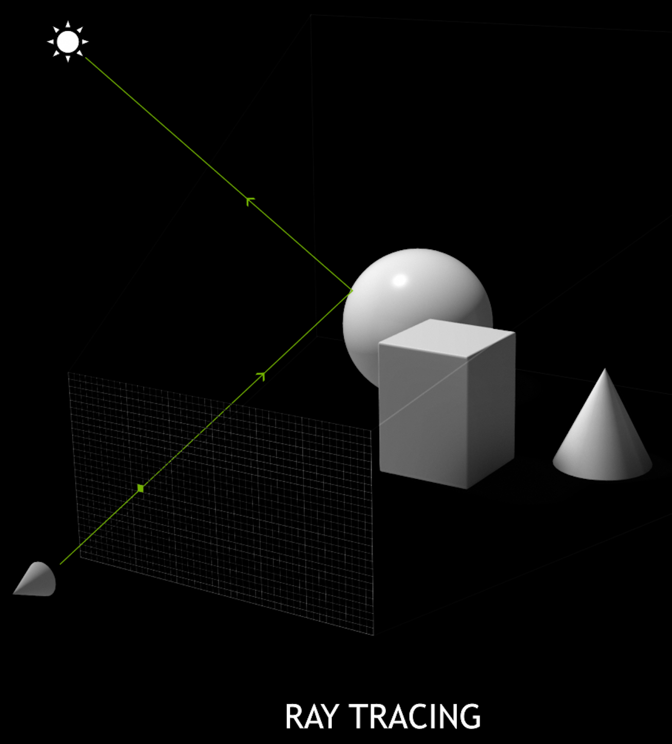
Raytrace Diagram
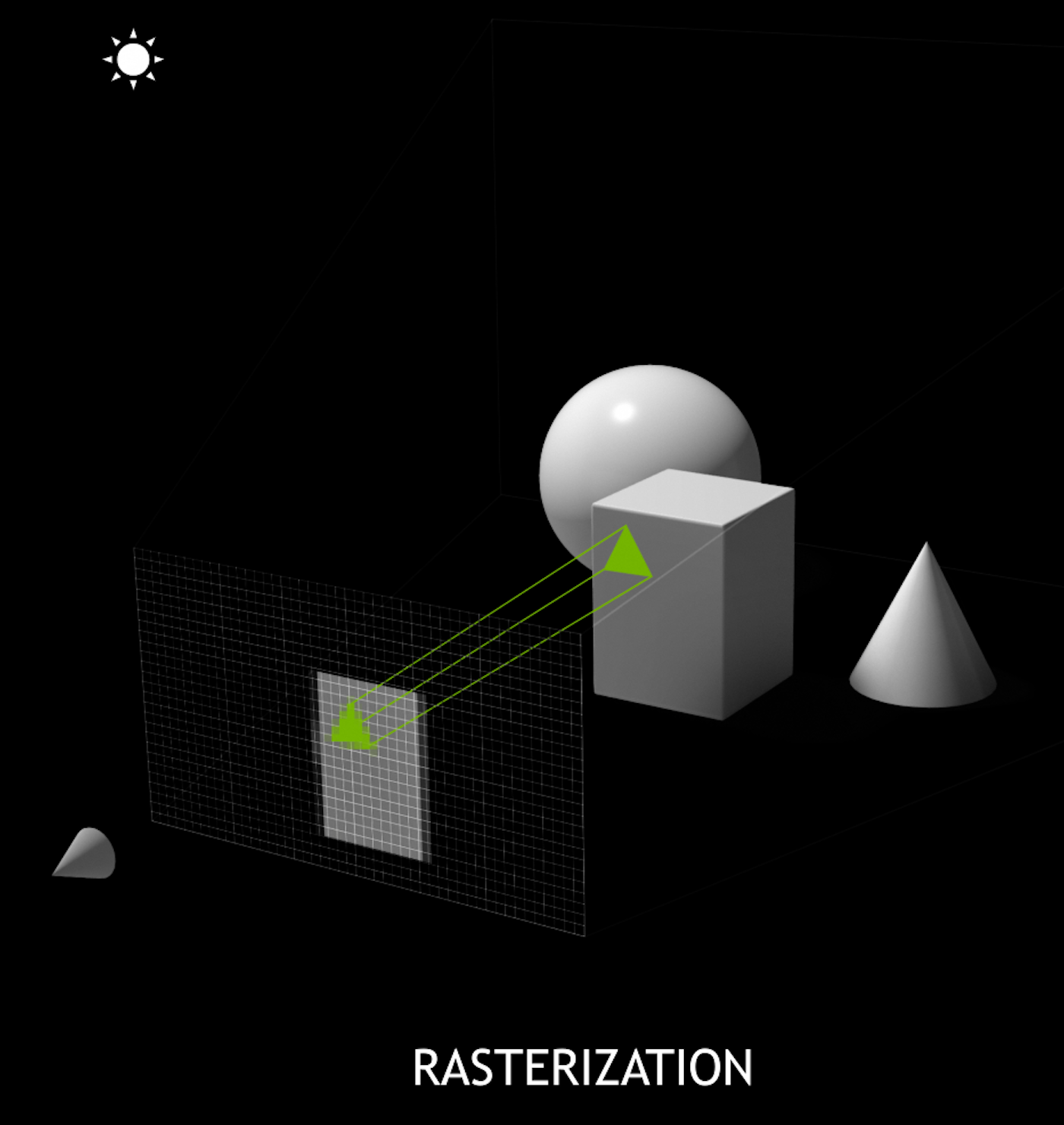
Ray-tracing vs Rasterization
Outline : Introducing the Tools

- Understanding GPUs
- Graphical Origins
- NVIDIA Turing GPU
- CPU vs GPU architectures
- Latency vs Throughput
- How to Make Effective Use of GPUs ?
- Use Higher Level Libraries -> Thrust
- Parallel / Simple / Uncoupled
- GPU Constraints -> Array-Oriented Design -> NumPy
- Serialization
- Serialization Benefits
- NumPy
- Foundation of Python Data Ecosystem
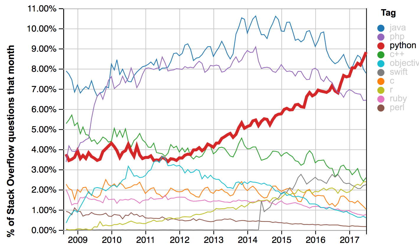
- Python : fastest growing major programming language ? Why ?
- NumPy Example : closest approach of Ellipse to a Circle
- NumPy Example : NLL Reconstruction fit : On one slide
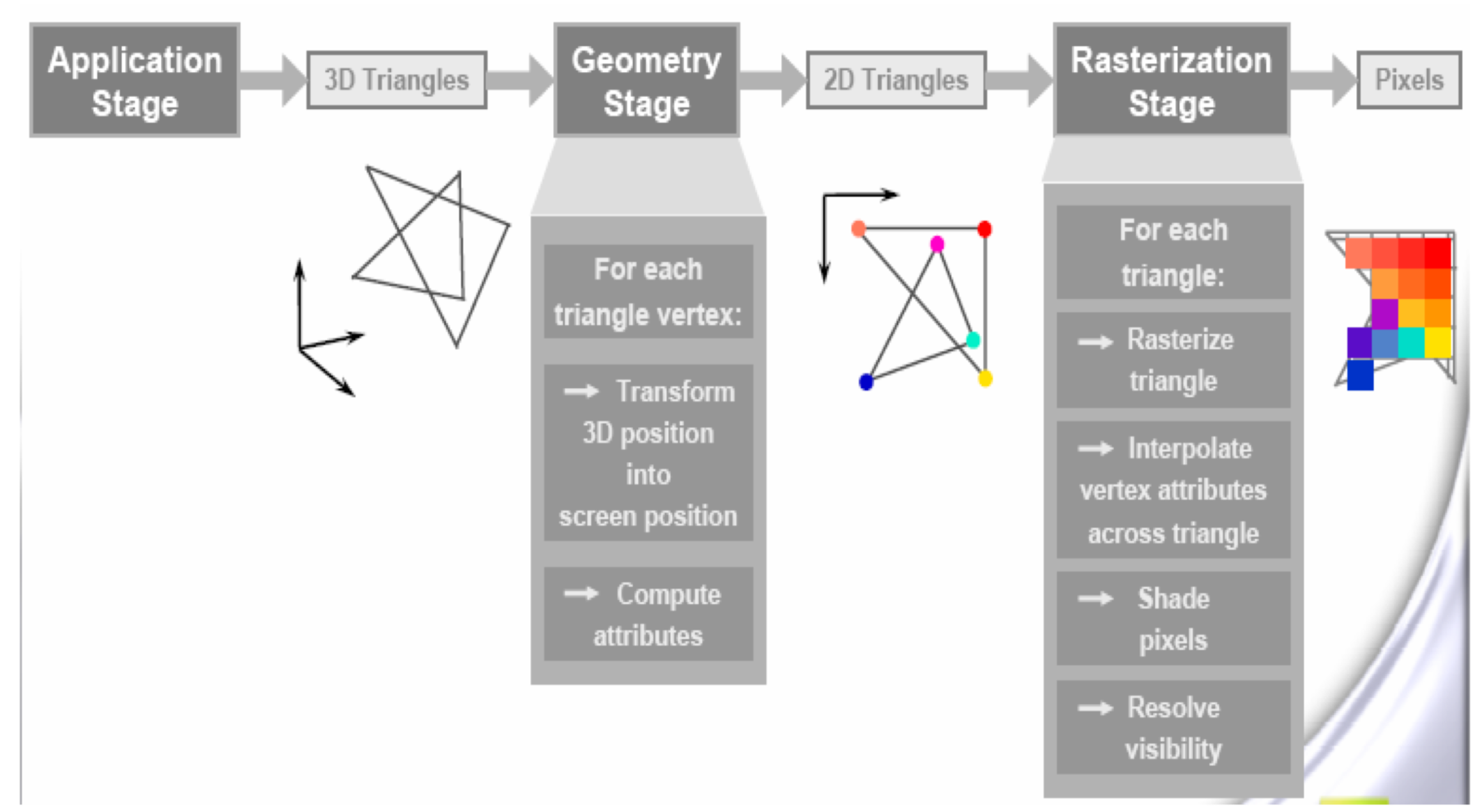
Understanding GPUs : Graphical Origins : An Extremely Parallel Problem
- GPUs evolved to rasterize 3D graphics, eg OpenGL graphics pipeline
- millions of triangles, millions of pixels, mostly independent
- simple data structures : vertices, triangles, pixels
- literally billions of small "shader" programs run per second
NVIDIA Turing GPU : 72 SM, 4608 CUDA cores
NVIDIA Turing GPU : 72 SM, 4608 CUDA cores (spec)
Thousands of CUDA cores
GPU : Turing TU102
- 72 Streaming Multiprocessors (SM)
- 4608 CUDA cores (64 per SM)
GPU : Volta V100 (eg Titan V)
- 80 SM
- 5120 CUDA cores (64 per SM)
CPU : Intel Xeon Processor Family
- Up to 28 cores, typically 8-18 cores
CPU vs GPU architectures, Latency vs Throughput
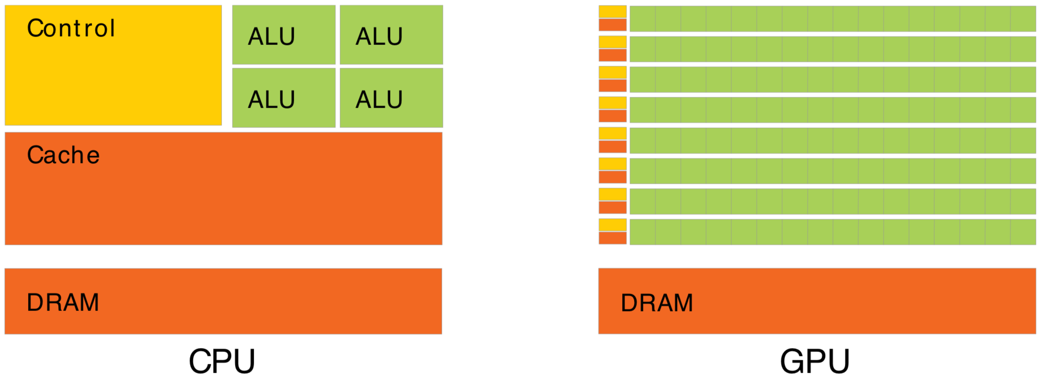
Waiting for memory read/write, is major source of latency...
- CPU : latency-oriented : Minimize time to complete single task : avoid latency with caching
- complex : caching system, branch prediction, speculative execution, ...
- GPU : throughput-oriented : Maximize total work per unit time : hide latency with parallelism
- many simple processing cores, hardware multithreading, SIMD (single instruction multiple data)
- simpler : lots of compute (ALU), at expense of cache+control
- design assumes abundant parallelism
Effective use of Totally different processor architecture -> Total reorganization of data and computation
Understanding Throughput-oriented Architectures https://cacm.acm.org/magazines/2010/11/100622-understanding-throughput-oriented-architectures/fulltext
How to Make Effective Use of GPUs ? -> Use Higher Level Libraries
High level C++ access to CUDA
"... Code at the speed of light ..."

"... high-level interface greatly enhances programmer productivity ..."
- https://developer.nvidia.com/Thrust
- header only library, comes with CUDA
- high-level abstraction : reduce, scan, sort
- rapid prototyping
- easy interop with CUDA
- Not many available, use if possible
- benefit from other peoples experience
- Thrust : high level C++ interface to CUDA
- OptiX : raytrace engine
- cuRAND, cuFFT, cuBLAS, cuSOLVER, ...
- CUB : http://nvlabs.github.io/cub/
https://developer.nvidia.com/gpu-accelerated-libraries

For adventurous early adopters
How to Make Effective Use of GPUs ? Parallel / Simple / Uncoupled
Optical Photon Simulation
- Abundant parallelism
- Many millions of photons
- Low register usage
- Simple optical physics, texture lookups
- Little/No synchronization
- Independent photons -> None
- Minimize CPU<->GPU copies
- geometry copied at initialization
- gensteps copied once per event
- only hits copied back
~perfect match for GPU acceleration
- Abundant parallelism
- many thousands of tasks (ideally millions)
- Low register usage : otherwise limits concurrent threads
- simple kernels, avoid branching
- Little/No Synchronization
- avoid waiting, avoid complex code/debugging
- Minimize CPU<->GPU copies
- reuse GPU buffers across multiple CUDA launches

How Many Threads to Launch ?
- can (and should) launch many millions of threads
- mince problems as finely as feasible
- maximum thread launch size : so large its irrelevant
- maximum threads inflight : #SM*2048 = 80*2048 ~ 160k
- best latency hiding when launch > ~10x this ~ 1M
Understanding Throughput-oriented Architectures https://cacm.acm.org/magazines/2010/11/100622-understanding-throughput-oriented-architectures/fulltext
NVIDIA Titan V: 80 SM, 5120 CUDA cores
GPU Constraints -> Array-Oriented Design -> NumPy
Serialization Benefits
- Persist everything to file -> fast development cycle
- geocache : initialize in seconds, not minutes
- interactive debug/analysis : NumPy,IPython
- flexible testing
- Can transport everything across network:
- production flexibility : distributed compute
- Arrays for Everything -> direct access debug
- (num_photons,4,4) float32
- (num_photons,16,2,4) int16 : step records
- (num_photons,2) uint64 : history flags
- (num_gensteps,6,4) float32
- (num_csgnodes,4,4) float32
- (num_transforms,3,4,4) float32
- (num_planes,4) float32
- (num_flightpath_views,4,4) float32
- ...
YET : Opticks libs do not depend on NumPy/python
- Separate address space -> Serialization
- upload/download : host(CPU)<->device(GPU)
- Serialize everything -> Arrays
- Many small tasks -> Arrays
- Order undefined -> Arrays
- Object-oriented
- mixes data and compute
- complicated serialization
- model complex systems, great up to ~1000 objects
- Array-oriented : ideal fit for GPU work
- separate data from compute, functional approach
- inherent serialization
- inherent simplicity, works for millions of items
- NumPy leading array-oriented package
- NumPy .npy : Simple Array Serialization Format
- metadata header : array shape and type
- read/write NumPy arrays from C++ https://github.com/simoncblyth/np/blob/master/NP.hh
NumPy : Foundation of Python Data Ecosystem
https://bitbucket.org/simoncblyth/intro_to_numpy
Very terse, array-oriented (no-loop) python interface to C performance
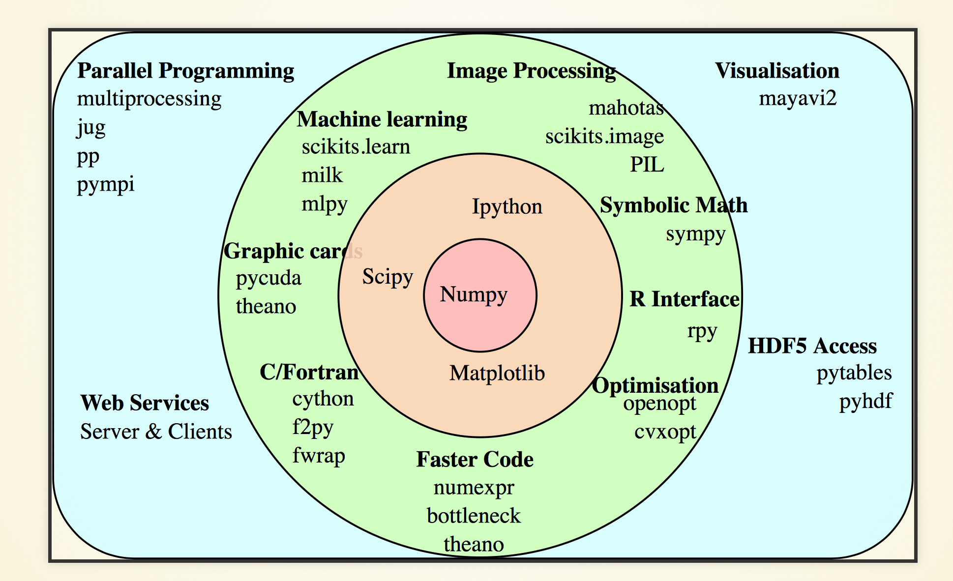
- C speed, python brevity + ease
- array-oriented
- vectorized : no python loops
- efficiently work with large arrays
- Recommended paper:
- The NumPy array: a structure for efficient numerical computation https://hal.inria.fr/inria-00564007
https://docs.scipy.org/doc/numpy/user/quickstart.html
http://www.scipy-lectures.org/intro/index.html
https://github.com/donnemartin/data-science-ipython-notebooks
Python : fastest growing major programming language : Why?
- Python more than doubled userbase over past five years (measured by Stackoverflow questions)
- Data science + machine learning developers prefer Python ? But why ?
- easy to learn, fast to write, fast to read
- efficient (no-copy) memory sharing between C/C++ libraries and scripts, due to Buffer Protocol
- easiest way to use Buffer Protocol (from Python and C) is via NumPy : so they all do:
- TensorFlow, Theano, Keras, Scikit-learn
https://stackoverflow.blog/2017/09/14/python-growing-quickly/
https://insights.stackoverflow.com/trends
https://jakevdp.github.io/blog/2014/05/05/introduction-to-the-python-buffer-protocol/
NumPy Example : closest approach of Ellipse to a Circle
import numpy as np

def ellipse_closest_approach_to_point( ex, ez, _c ):
    """ex, ez: ellipse semi-axes, c: coordinates of point in ellipse frame"""
    c = np.asarray( _c )  ; assert c.shape == (2,)

    t = np.linspace( 0, 2*np.pi, 1000000 )      # t: array of 1M angles [0,2pi]
    e = np.zeros( [len(t), 2] )
    e[:,0] = ex*np.cos(t)
    e[:,1] = ez*np.sin(t)                       # e: 1M parametric [x,z] points on the ellipse

    return  e[np.sum((e-c)**2, axis=1).argmin()]    # point on ellipse closest to c
| expression | shape | note |
|---|---|---|
| e | (1000000,2) | |
| c | (2,) | |
| e-c | (1000000,2) | c is broadcast over e : must be compatible shape |
| np.sum((e-c)**2, 1) | (1000000,) | axis=1 : summing over the axis of length 2 |
| np.sum((e-c)**2, 0) | (2,) | axis=0 : summing over axis of length 1M |
| np.sum((e-c)**2, None) | () | axis=None : summing over all elements, yielding scalar |
https://bitbucket.org/simoncblyth/opticks/src/tip/ana/x018_torus_hyperboloid_plt.py
NumPy Example : NLL Reconstruction fit : On one slide
Array-oriented brevity : prototyping
- introspect interactively with IPython
- follow shape at every stage
In [5]: t_model([0,0,0])
Out[5]: array([10., 10., 10., ..., 10., 10., 10.])

In [6]: t_model([0,0,0]).shape
Out[6]: (2500,)

In [7]: t.shape
Out[7]: (2500,)

In [8]: t
Out[8]: array([ 6.783 ,  5.4754,  6.1462, ... ])
##!/usr/bin/env python
import numpy as np, scipy.stats as st, scipy.optimize as so
np.random.seed(0)  # reproducibility

# generate n*n (x,y,z) coordinates on a sphere
n = 50
u,v = np.meshgrid( np.linspace(0,np.pi,n+2)[1:-1],
                   np.linspace(0,2*np.pi,n+1)[:-1] )
uu = u.ravel() ; vv = v.ravel()
sph = np.zeros( [len(uu), 3] )
sph[:,0] = np.sin(uu)*np.cos(vv)
sph[:,1] = np.sin(uu)*np.sin(vv)
sph[:,2] = np.cos(uu)
R = 10  ; sph *= R

# mockup "truth" position
parTru = np.array( [0,0,R/2, 1] )

# distances from all the sphere coordinates to the "truth" position
d = np.sqrt(np.sum((sph - parTru[:3])**2, axis=1 ))

# mockup a time linear with the distance with a normal smearing
t = d + parTru[3]*np.random.randn(len(d))

# geometric "time" as function of position
t_model = lambda par:np.sqrt(np.sum((sph - par[:3])**2, axis=1 ))

# Assumed PDF of "time" at each sphere position, normal around geometric time with some sigma.
NLL = lambda par:-np.sum( st.norm.logpdf(t, loc=t_model(par), scale=par[3] ))

parIni = np.array( [0,0,0,1] )  # initial parameter values
parFit = so.minimize(NLL, parIni, method='nelder-mead').x ; print(parFit)
https://bitbucket.org/simoncblyth/intro_to_numpy/src/default/recon_terse.py
Outline of Techniques : Monte Carlo Method

- Technique : Monte Carlo Method
- apply randomness to model complex systems
- optical photon simulation, deciding history
- sampling using Cumulative Distribution Function
- modelling Scintillator Re-emission
- modelling Scattering and Absorption
- accept-reject sampling
- estimating pi
- Technique : NVIDIA CUDA + Thrust
- GPU estimating pi
- NLL Fitting Extended Example : CPU+GPU techniques
- Geant4 : Standard Monte Carlo in HEP
- simulation toolkit generality
- overview
Monte Carlo Method : apply randomness to model complex systems
Casino de Monte-Carlo, Monaco (French Riviera)

- named after city famous for casinos
- prior to computers : roulette wheel was a convenient RNG
- developed 1940s for neutron transport (Ulam, von Neumann) using first general purpose computer
Simulate designs before building them
Generate history of a system using random sampling techniques making variables follow expected PDFs[1]
- uniform random numbers [0,1] are mapped to probabilities
- applicable to problems too complex for an analytic solution
- ubiquitous : physics/biology/engineering/finance/climate/...
- eventually validate against real data measurements
- hopefully find problems : improve models (PDFs)
simulation is vital to understand/design anything complex
[1] PDFs : probability density functions
https://www.slideserve.com/hafwen/monte-carlo-detector-simulation Pat Ward, Cambridge University, 74 pages Powerpoint
Optical Photon Simulation : Deciding history on way to boundary
Possible Histories
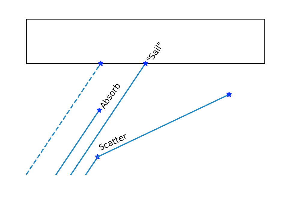
- optical photon simulation straightforward : as only a few processes
- BUT : principals are the same as full MC
- intersect ray with geometry -> distance to boundary
- lookup absorption length, scattering length for material
depending on wavelength
- Opticks uses GPU texture interpolation
- "role dice" : characteristic lengths -> stochastic distances
Pick winning process from smallest distance
boundary_distance = from_geometry  # no random number needed
absorption_distance = -absorption_length * ln(u0)
scattering_distance = -scattering_length * ln(u1)
## u0, u1 uniform randoms in [0,1] : distances always +ve
If scatter:
- pick new photon direction at random
- set polarization perpendicular to new direction (transverse) and in same plane as direction and initial polarization
- rejection-sampling used to pick new polarization such that angle between old and new follows cos^2 distribution
- then repeat from 1.
Theory (eg Rayleigh scattering) -> PDFs used in the simulation
https://bitbucket.org/simoncblyth/opticks/src/default/optixrap/cu/propagate.h https://bitbucket.org/simoncblyth/opticks/src/default/optixrap/cu/rayleigh.h
MC Method : Sampling using Cumulative Distribution Function (CDF)
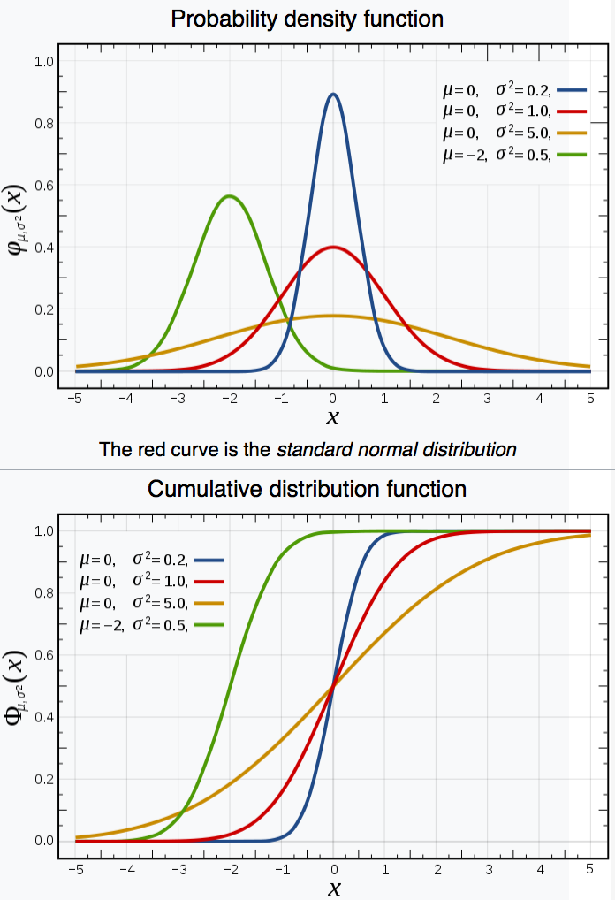
Aim : create sample (a set of values) that follows an analytic PDF
Cumulative distribution function (CDF) : Prob( X < x)
- definite integral PDF f -> CDF F
- F(b) - F(a) = P( a < X <= b ) = Integral a->b f(x) dx
- monotonically increasing function, CDF(-inf) = 0, CDF(inf) = 1
Map uniform randoms onto probabilities
- integrate PDF -> CDF (mapping PDF domain onto probability [0,1] )
- invert the CDF, so domain becomes [0,1]
- inverted_CDF(uniform random) -> sample value
Intuitively : throw randoms uniformly "vertically"
- Sigmoid CDF : low probability close to zero or 1 corresponding to tails
- greater probability in high PDF areas
- extreme case of delta-function PDF : all probability at one value
- sigmoid CDF becomes Heaviside step-function
CDF "encodes" shape of PDF in convenient form for sampling
Monte Carlo Method : Modelling Scintillator Re-emission
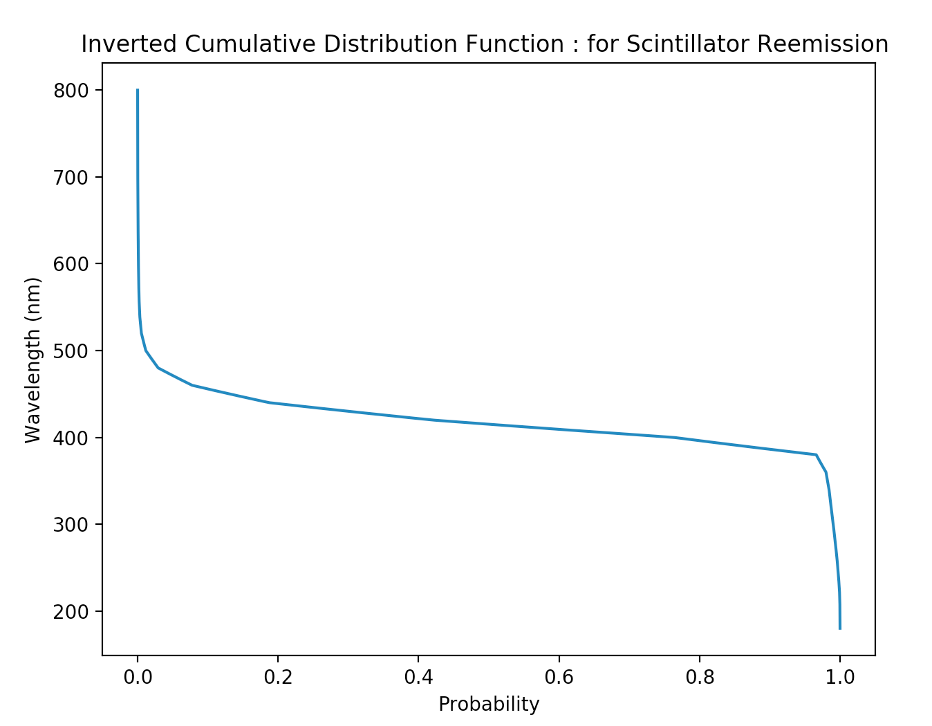
- reemission_probability(wavelength)
- fraction of light absorbed in scintillator re-emitted with different wavelength.
- generating re-emitted wavelength
- expected PDF(wavelength) -> inverted_CDF(probability)
Opticks Re-emission model
- fraction of absorbed photons "reincarnated" in same thread
- inverted_CDF(probability) -> GPU "re-emission" texture
float uniform_sample_reemit = curand_uniform(&rng);
if (uniform_sample_reemit < reemission_probability )
{
    ...
    p.wavelength = reemission_lookup(curand_uniform(&rng));    # re-emission texture lookup
    s.flag = BULK_REEMIT ;
    return CONTINUE;
}
else
{
    s.flag = BULK_ABSORB ;
    return BREAK;
}
https://bitbucket.org/simoncblyth/opticks/src/default/optixrap/cu/propagate.h
Monte Carlo Method : Modelling Scattering and Absorption
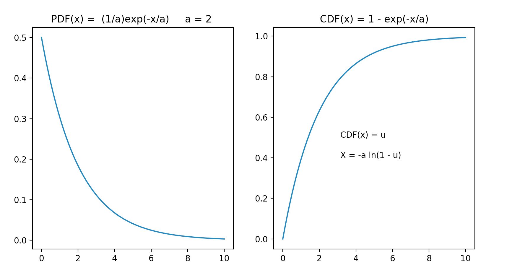
Create sample with exponential PDF, using CDF
- PDF(x) = (1/a) exp(-x/a)
- CDF(x) = 1 - exp(-x/a)
- a
- characteristic scale of process, eg decay time or scattering/absorption/attenuation length
- u
- uniform random value in [0,1] ; 1-u equivalent to u
Known analytic form of CDF, means simple sampling:
Equate CDF probability with uniform random value [0,1]
- CDF(x) = 1 - exp(-x/a) = u
- exp(-x/a) = 1 - u
- X = -a ln(1-u)
- X = -a ln(u)
- X
- stochastic distance/time obtained from characteristic scale a and uniform random u
https://www.eg.bucknell.edu/~xmeng/Course/CS6337/Note/master/node50.html
Monte Carlo Method : Accept-Reject Sampling
Simple technique providing a sample that follows a distribution. Example PDF : pdf(x) = (3/8).( 1 + x^2 )
- scatter random points (x,y) across PDF graph (piecewise for better efficiency)
- accept x for pdf(x) < y : implement in C++ with do { } while ( condition )
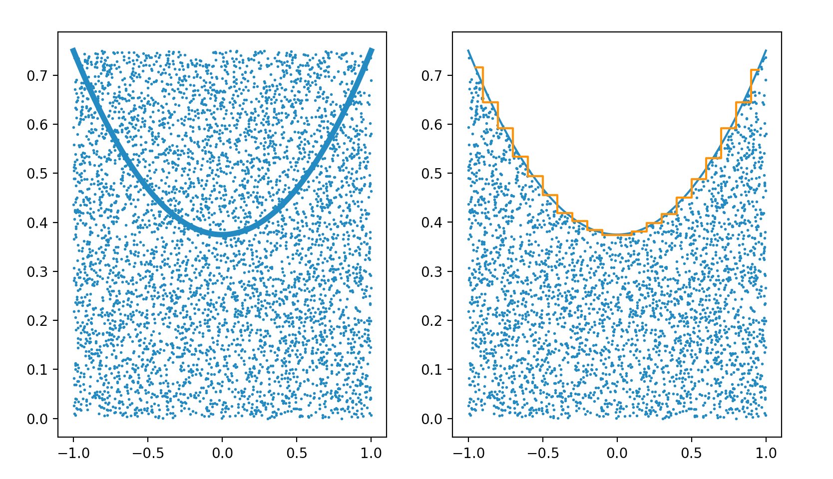
https://bitbucket.org/simoncblyth/intro_to_numpy/src/default/accept_reject_sampling.py
Monte Carlo Method : Accept-Reject Sampling (NumPy Code in IPython)
in [1]: import numpy as np
In [2]: a = np.random.rand( 1000000,2 )       # 2M random floats uniform in [0,1]

In [3]: a[:,0] = a[:,0]*2. - 1.   #  [0,1] -> [-1,1]
In [4]: a[:,1] = a[:,1]*0.75      #  [0,1] -> [0,0.75]     pdf(0) = pdf(1) = 0.75

In [5]: pdf = lambda x:(3./8.)*(1+x**2)         # simple symmetric PDF normalized on -1:1

In [6]: w = np.where( a[:,1] < pdf(a[:,0]) )     # indices of accepted sample

In [7]: s = a[w][:,0]                     # accepted sample of 666301 values

In [8]: s
Out[8]: array([ 0.0382,  0.9755,  0.6855, ...,  0.5962,  0.9094, -0.8292])

In [9]: s.shape
Out[9]: (666301,)

In [10]: a.shape
Out[10]: (1000000, 2)

In [11]: a
Out[11]:
array([[ 0.0382,  0.0752],
       [ 0.9755,  0.0495],
       [ 0.6855,  0.1835],
       ...,
       [ 0.5837,  0.7297],
       [-0.7534,  0.7253],
       [-0.8292,  0.0019]])
https://bitbucket.org/simoncblyth/intro_to_numpy/src/default/accept_reject_sampling.py
MC Method : Estimating Pi from circle/square count ratio : pi r^2/(2r)^2
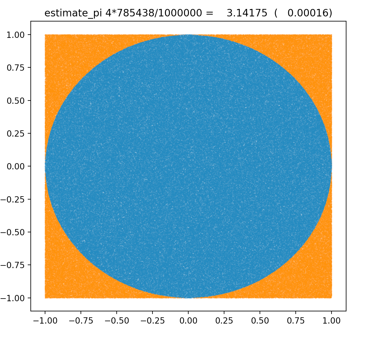
https://bitbucket.org/simoncblyth/intro_to_numpy/src/default/estimate_pi.py
Monte Carlo Method : Estimating Pi : NumPy Code in IPython
In [1]: from __future__ import division     # python3 style default
In [2]: import numpy as np

In [3]: a = np.random.rand( 1000000,2 )     # 2M uniform [0,1] random floats

In [4]: a[:,0] = a[:,0]*2. - 1.             # NB: no loops at python level

In [5]: a[:,1] = a[:,1]*2. - 1.

In [6]: mask = np.sum(a*a,1) < 1            # mask : array of booleans with same shape as a

In [7]: w = np.where(mask)                  # w : array of indices of a within the mask

In [8]: epi = 4*len(w[0])/len(a)            # estimate of pi =  4*(cicle count)/(square count)

In [9]: label = " estimate_pi 4*%d/%d = %10.5f  (%10.5f) " % (len(w[0]), len(a), epi, epi-np.pi )

In [10]: a.shape
Out[10]: (1000000, 2)

In [11]: a[w].shape                         # shape of the selection
Out[11]: (785209, 2)

In [12]: a[w]                              # select via an array of indices
Out[12]:
array([[-0.3253,  0.8069],
       [ 0.2202, -0.8232],
       [-0.9173, -0.088 ],
       ...,
       [ 0.1739, -0.1885],
       [-0.1812, -0.8979],
       [ 0.4604, -0.524 ]])
https://bitbucket.org/simoncblyth/intro_to_numpy/src/default/estimate_pi.py
Thrust : Estimate pi : operator() method runs on device (GPU)
- C++ functor with __device__ float operator()
- struct member N set on host(CPU), used on device(GPU) : taken care of by Thrust
- https://bitbucket.org/simoncblyth/intro_to_cuda
##include <curand_kernel.h>

struct estimate_pi
{
    estimate_pi(int _N) : N(_N) {}

    __device__ float operator()(unsigned seed)
    {
        float sum = 0;
        curandState rng;
        curand_init(seed, 0, 0, &rng);
       // initializing curand is very expensive better to split/persist/load, see next pages

        for(int i = 0; i < N; ++i)
        {
            float x = curand_uniform(&rng);
            float y = curand_uniform(&rng);
            float dist = sqrtf(x*x + y*y);
            if(dist <= 1.0f) sum += 1.0f;
        }
        sum *= 4.0f;
        return sum / N;
    }

    int N ;
};
https://bitbucket.org/simoncblyth/intro_to_cuda/src/default/thrust_curand_estimate_pi.cu
Thrust : Estimate pi : thrust::transform_reduce does the "launch"
##include <thrust/iterator/counting_iterator.h>
##include <thrust/transform_reduce.h>
##include <iostream>
##include <iomanip>

int main()
{
     int N = 10000; int M = 30000;

     float estimate = thrust::transform_reduce(            // NB functor call ordering is undefined
                thrust::counting_iterator<int>(0),
                thrust::counting_iterator<int>(M),   // 1st two args define implicit sequence
                estimate_pi(N),                      // the functor to apply to the sequence
                0.0f,                                // initial value of reduction
                thrust::plus<float>())/M ;           // how to combine results from the functor call

      std::cout
          << " M " << M << " N " << N
          << std::setprecision(5) << std::fixed
          << " estimate " << estimate
          << " delta "   << estimate - M_PI << std::endl ;

      return 0;
}
epsilon:tests blyth$ nvcc thrust_curand_estimate_pi.cu
epsilon:tests blyth$ ./a.out
 M 30000 N 10000 estimate 3.14142 delta -0.00017
cuRAND Random Number Generation : Split Initialization and Usage
https://bitbucket.org/simoncblyth/intro_to_cuda/src/tip/rng/rng_states.cu
Persistent CUDA Context
GPU buffers live within CUDA context
- load once at initialization
- reuse for multiple kernel launches
Opticks populates context at initialization:
- random number generator RNG (curandState)
- Geometry : CSG Nodes/Transforms/Vertices/...
Concurrent generation of millions of reproducible sequences of pseudorandom numbers
- sub-sequences assigned to each photon index
- curandState maintains position in sub-sequences
curand_init very expensive -> huge performance hit:
- not just time to initialize
- ALSO : large stack -> limits number of concurrent threads
Solution:
- split initialization into separate launch(es)
- do once only, at install time : persist state to installcache
- fixes maximum photon launch size : currently 3M threads
- load rng_state into CUDA context at executable initialization, together with geometry
- subsequent CUDA launches, eg for each event
- small stacksize, lightweight threads -> generate randoms without initializing, increment rng_state
Understanding this technicality -> correct "mental model" of CUDA context
NLL Fitting Extended Example : Demo CPU+GPU project techniques
Hiding the CUDA implementation
// recon/Rec.hh // requires nvcc compilation
##include "NLL.hh"
template<typename T>
T Rec<T>::nll_() const
{
    return -thrust::transform_reduce(
              thrust::make_counting_iterator(0),
              thrust::make_counting_iterator(tnum),
              *nll, // NLL functor
              T(0),
              thrust::plus<T>()
           );
}
// recon/Recon.hh // gcc/clang/nvcc compilation
##include <vector>
template <typename T> struct Rec ;
template <typename T>
struct Recon
{
    Rec<T>* rec ; // <-- CUDA imp hidden behind pointer
    Recon( const char* dir ) ;
    T nll( const std::vector<T>& par );
};
https://bitbucket.org/simoncblyth/intro_to_cuda/src/tip/recon/
1. CPU+GPU Libs, Bridging header pattern
- GPU code library (nvcc) : NLL method
- CPU library + executable (gcc/clang) : Minuit2 fitter
- Recon.hh
- hides CUDA implementation behind Rec<T> pointer
2. NumPy array read/write from C++/CUDA C/Thrust
- develop in C++/CUDA C/Thrust
- debug with IPython/NumPy
3. Thrust : GPU development
- simplified : CPU<->GPU copy, memory management
- high level thrust::transform_reduce with functor
Real CUDA usage -> two compilers -> interop techniques required
Geant4 : Monte Carlo Simulation Toolkit
Geant4 : Monte Carlo Simulation Toolkit Generality
Standard Simulation Tool of HEP
Geant4 simulates particles travelling through matter
- high energy, nuclear and accelerator physics
- medical physics : deciding radiotherapy doses/sources
- space engineering : satellites
Geant4 Approach
- geometry : tree of CSG solids
- particles : track position and time etc..
- processes : nuclear, EM, weak, optical
Very General and Capable Tool
- mostly unused for optical photon propagation
Geant4 : Overview
No main(), No defaults
Geant4 is a toolkit : it provides no main()
Materials and surfaces can be assigned optical properties such as: RINDEX, REFLECTIVITY
- very flexible model
- every optical photon represented as G4Track : pushed and popped from stack
Initialization
- define heirarchy of volumes, with materials, surfaces
- physics particles and processes defined
- setup primary particle generation to be used for each event
Beginning of Run
- geometry optimized for navigation
- cross-section tables calculated for materials/cuts
Beginning of Event
- primary tracks are generated and pushed onto stack
- physics processes of tracks can create secondary tracks
- when stack empty, processing over
At Each Step of a Track
- all applicable processes "compete" : proposing physical interaction lengths (PIL)
- shortest PIL "wins" (limits the step and that process can generate secondary tracks and change the primary track)
60 slide intro from one of the primary Geant4 architects/developers
http://geant4.in2p3.fr/2005/Workshop/ShortCourse/session1/J.Apostolakis.pdf
Outline of Opticks : Problem, Solution, Geometry, Validation

- Optical Photon simulation problem, hybrid solution : Geant4 + Opticks
- Ray Traced Image Synthesis ≈ Optical Photon Simulation
- NVIDIA OptiX Ray Tracing Engine
- BVH : Boundary Volume Hierarchy
- BVH Pascal : software emulation
- BVH Turing : hardware "RT Cores"
- Primitives
- GPU Geometry starts from ray-primitive intersection
- Torus : much more difficult/expensive than other primitives
- CSG : Constructive Solid Geometry modelling
- Shapes defined "by construction"
- Which primitive intersect to pick ?
- Ray intersection with general CSG binary trees, on GPU
- Complete Binary Tree Serialization -> simplifies GPU side
- Evaluative CSG intersection Pseudocode : recursion emulated
- CSG Deep Tree : JUNO "fastener", balancing reduces tree height: 11 -> 4
- Geometry visualizations : Daya Bay Near Site, JUNO Central Detector
- CSG : (Cylinder - Torus) PMT neck : spurious intersects
- CSG : Alternative PMT neck designs
- Translation
- Auto-Instancing
- Opticks : translates G4 geometry to GPU, without approximation
- Opticks : Export of G4 geometry to glTF 2.0
- Opticks : translates G4 optical physics to GPU
- Validation : Opticks/G4 statistical comparison
- Simple Lights/Geometries
- 1M Rainbow S-Polarized
- Random Aligned Validation -> direct comparison
- Take Control of Geant4 Random Number Generator (RNG)
- Aligning CPU and GPU Simulations
- Direct comparison of GPU/CPU NumPy arrays
- Coincident Faces are Primary Cause of Issues : Spurious Intersects
- Summary
Optical Photon Simulation Problem...
JPMT Before Contact 2
Optical Photon Problem
- Cosmic muon backgrounds
- many millions of optical photons in JUNO scintillator
- Simulation Bottleneck
- ~99% CPU time, memory constraints
- Optical photons : naturally parallel, simple :
- produced by Cerenkov+Scintillation
- yield only Photomultiplier hits
-> Hybrid Solution : Geant4 + Opticks
Ray Traced Image Synthesis ≈ Optical Photon Simulation
Not a Photo, a Calculation
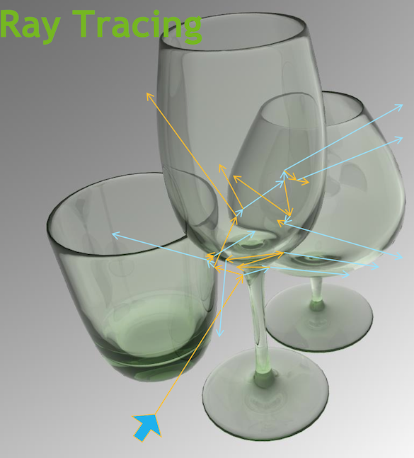
Geometry, light sources, optical physics ->
- pixel values at image plane
- photon parameters at detectors (eg PMTs)
Ray tracing has many applications :
- advertising, design, entertainment, games,...
- BUT : most ray tracers just render images
Ray-geometry intersection
- hw+sw continuously optimized over 30 years
- NVIDIA : "10+ Giga-ray intersections per second per GPU" (Turing GPU : hardware BVH acceleration )
- ray tracing
- cast rays thru image pixels into scene, recursively reflect/refract at intersects, combine returns into pixel values
- rasterization
- project 3D primitives onto 2D image plane, combine fragments into pixel values
NVIDIA® OptiX™ Ray Tracing Engine -- http://developer.nvidia.com/optix
OptiX Raytracing Pipeline
Analogous to OpenGL rasterization pipeline:
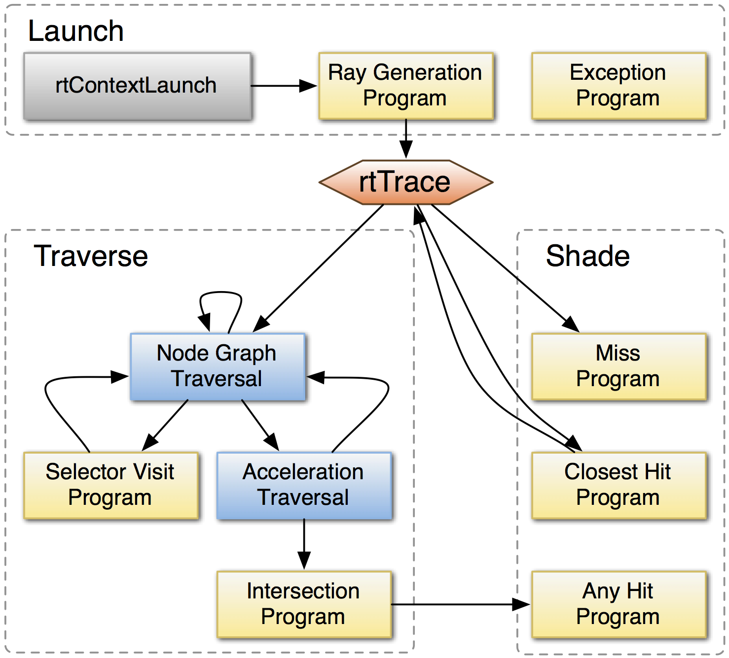
OptiX makes GPU ray tracing accessible
- accelerates ray-geometry intersections
- simple : single-ray programming model
- "...free to use within any application..."
NVIDIA expertise:
- ~linear scaling with CUDA cores across multiple GPUs
- acceleration structure creation + traversal (Blue)
- instanced sharing of geometry + acceleration structures
- compiler optimized for GPU ray tracing
- regular updates, profit from new GPU features:
- NVIDIA RTX™ with Volta, Turing GPUs
https://developer.nvidia.com/rtx
User provides (Yellow):
- ray generation
- geometry bounding box, intersects
BVH
BVH Pascal
BVH Turing
Opticks : GPU Geometry starts from ray-primitive intersection
- 3D parametric ray : ray(x,y,z;t) = rayOrigin + t * rayDirection
- implicit equation of primitive : f(x,y,z) = 0
- -> polynomial in t , roots: t > t_min -> intersection positions + surface normals
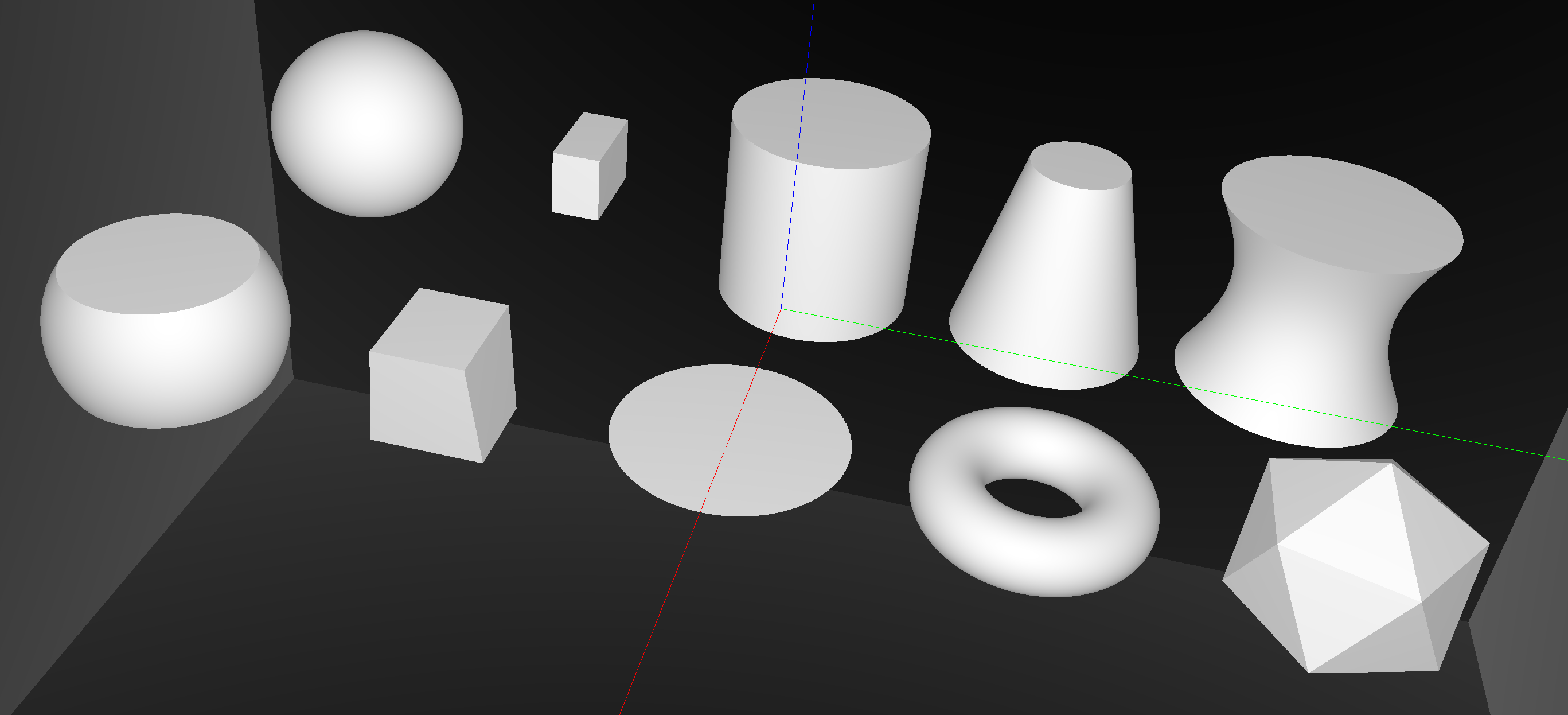
CUDA/OptiX intersection for ~10 primitives -> Exact geometry translation
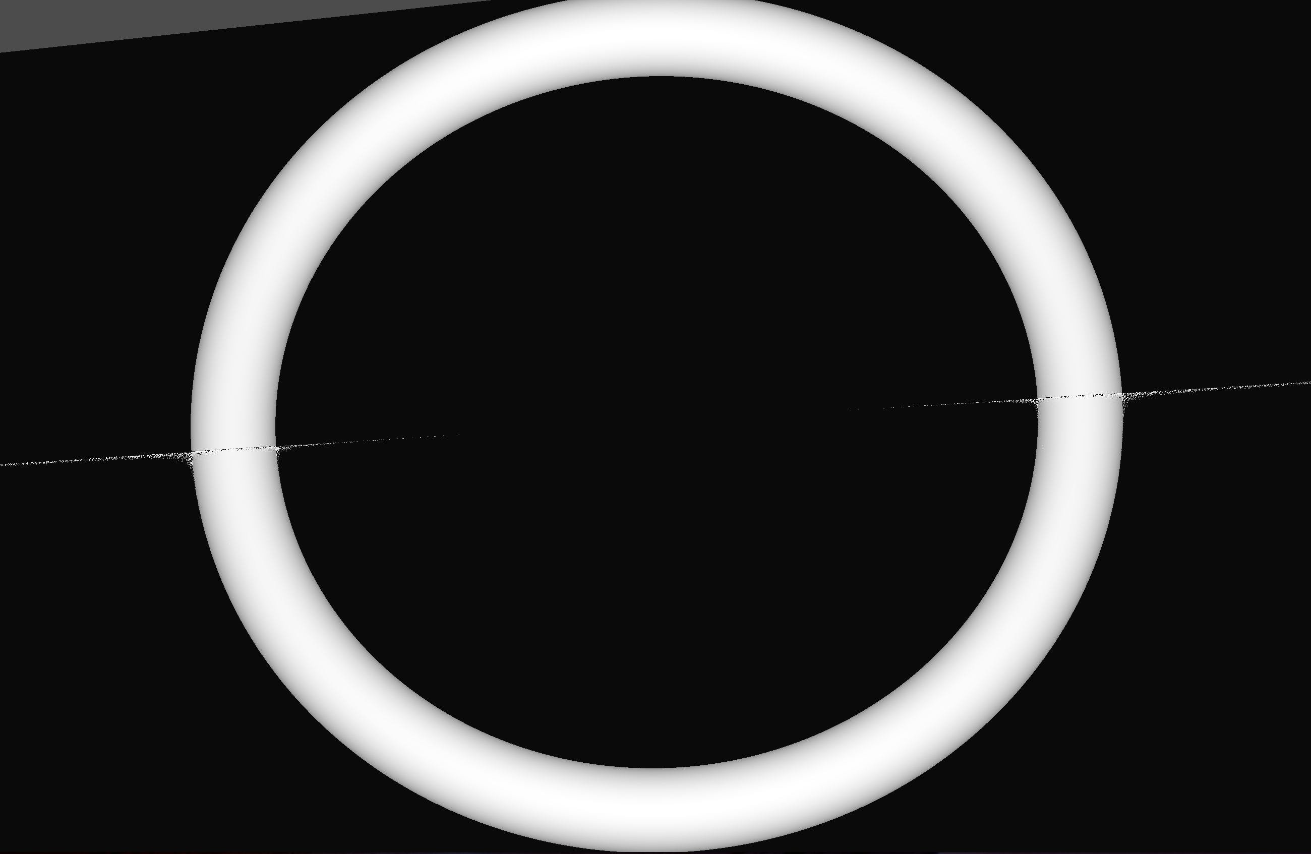
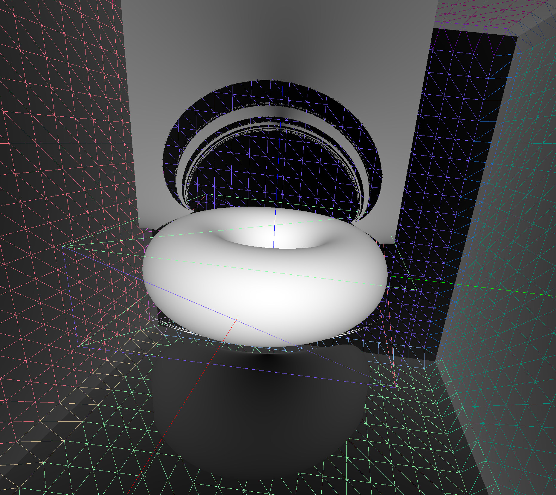
Torus : much more difficult/expensive than other primitives
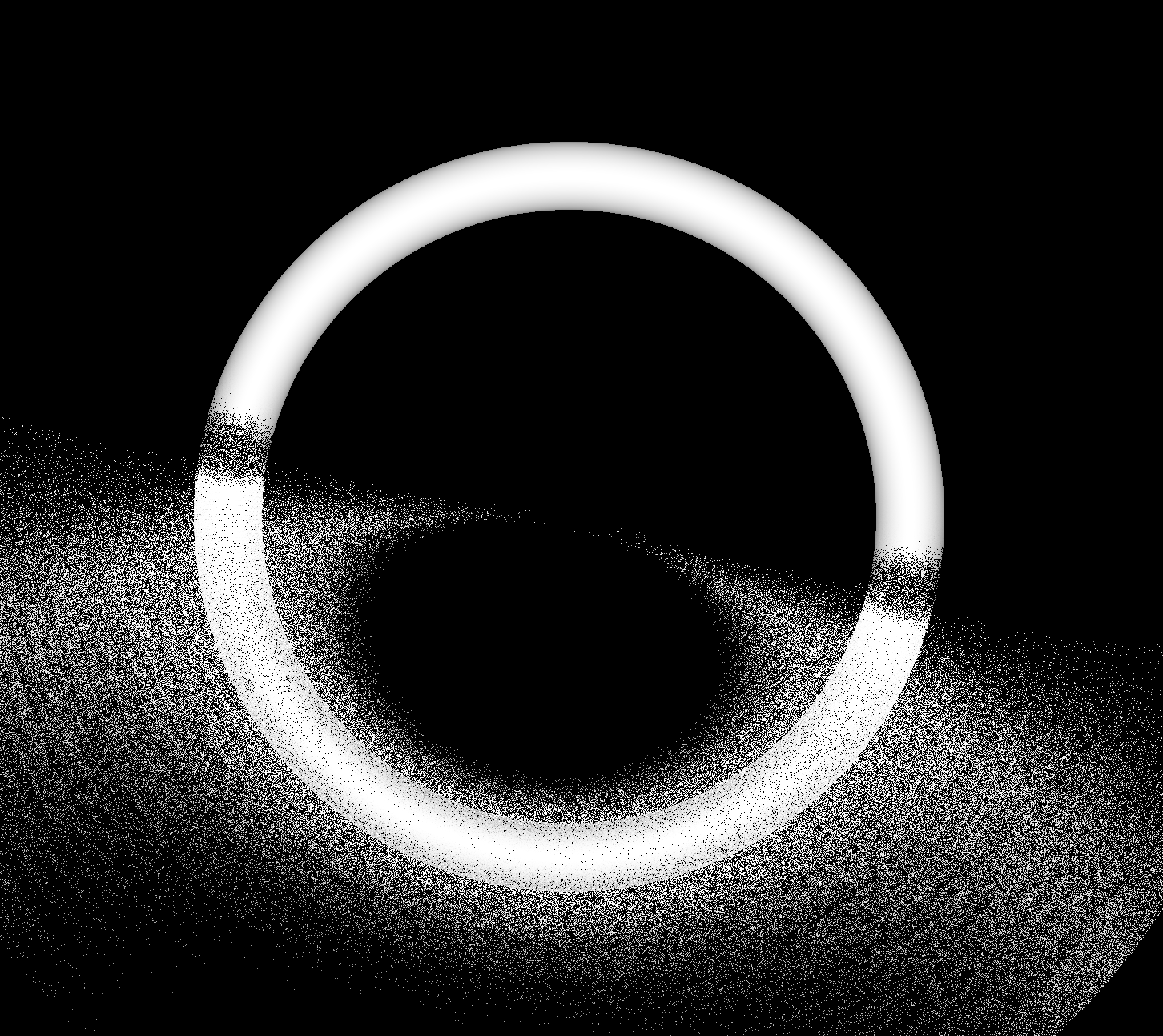
Torus artifacts


3D parametric ray : ray(x,y,z;t) = rayOrigin + t * rayDirection
- ray-torus intersection -> solve quartic polynomial in t
- A t^4 + B t^3 + C t^2 + D t + E = 0
High order equation
- very large difference between coefficients
- varying ray -> wide range of coefficients
- numerically problematic, requires double precision
- several mathematical approaches used
Best Solution : replace torus
- eg model PMT neck with hyperboloid, not cylinder-torus
Torus : different artifacts as change implementation/params/viewpoint
- Only use Torus when there is no alternative
- especially avoid CSG combinations with Torus

Constructive Solid Geometry (CSG) : Shapes defined "by construction"
CSG Binary Tree
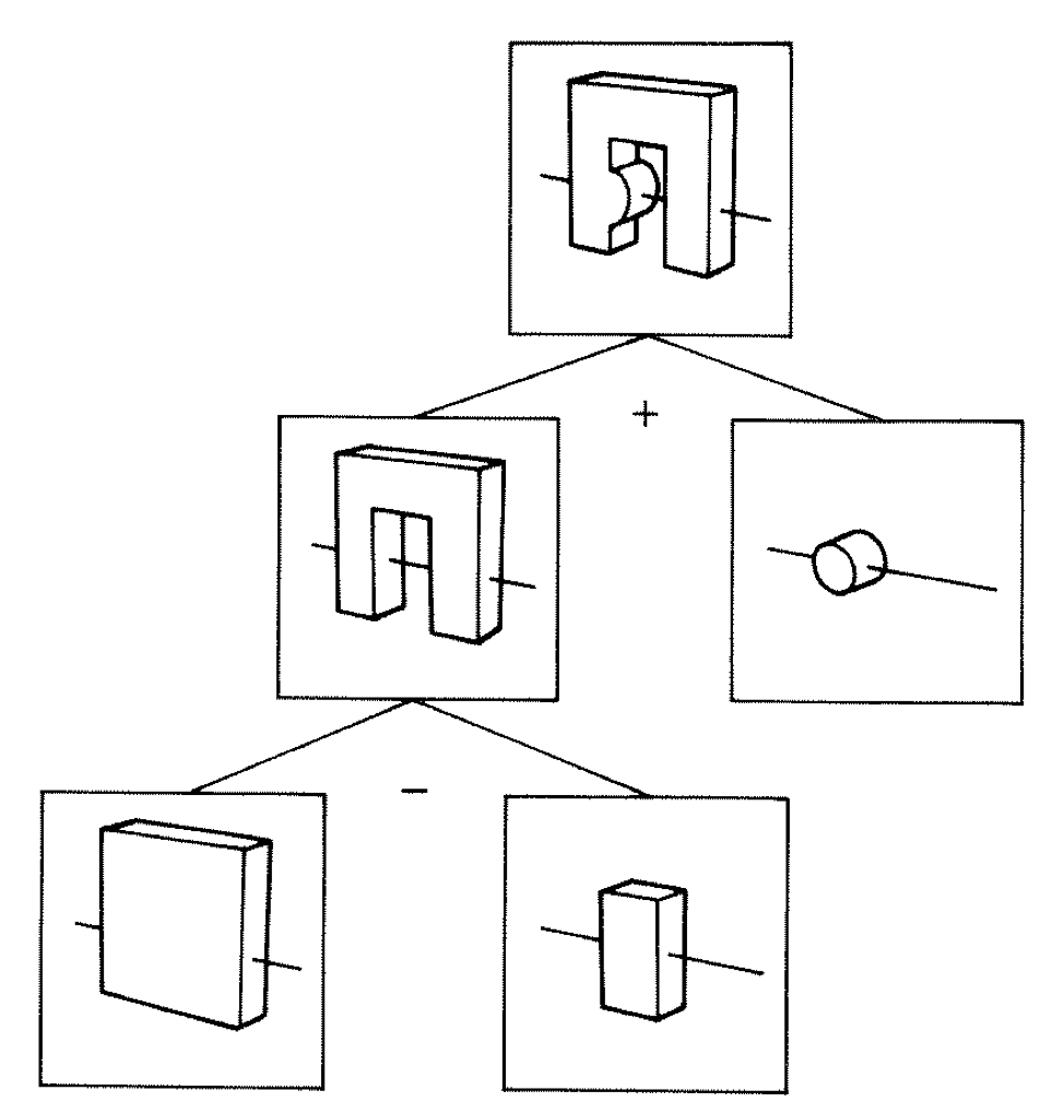
Primitives combined via binary operators
Simple by construction definition, implicit geometry.
- A, B implicit primitive solids
- A + B : union (OR)
- A * B : intersection (AND)
- A - B : difference (AND NOT)
- !B : complement (NOT) (inside <-> outside)
CSG expressions
- non-unique: A - B == A * !B
- represented by binary tree, primitives at leaves
3D Parametric Ray : ray(t) = r0 + t rDir
Ray Geometry Intersection
- primitive : find t roots of implicit eqn
- composite : pick primitive intersect, depending on CSG tree
How to pick exactly ?
CSG : Which primitive intersect to pick ?
In/On/Out transitions
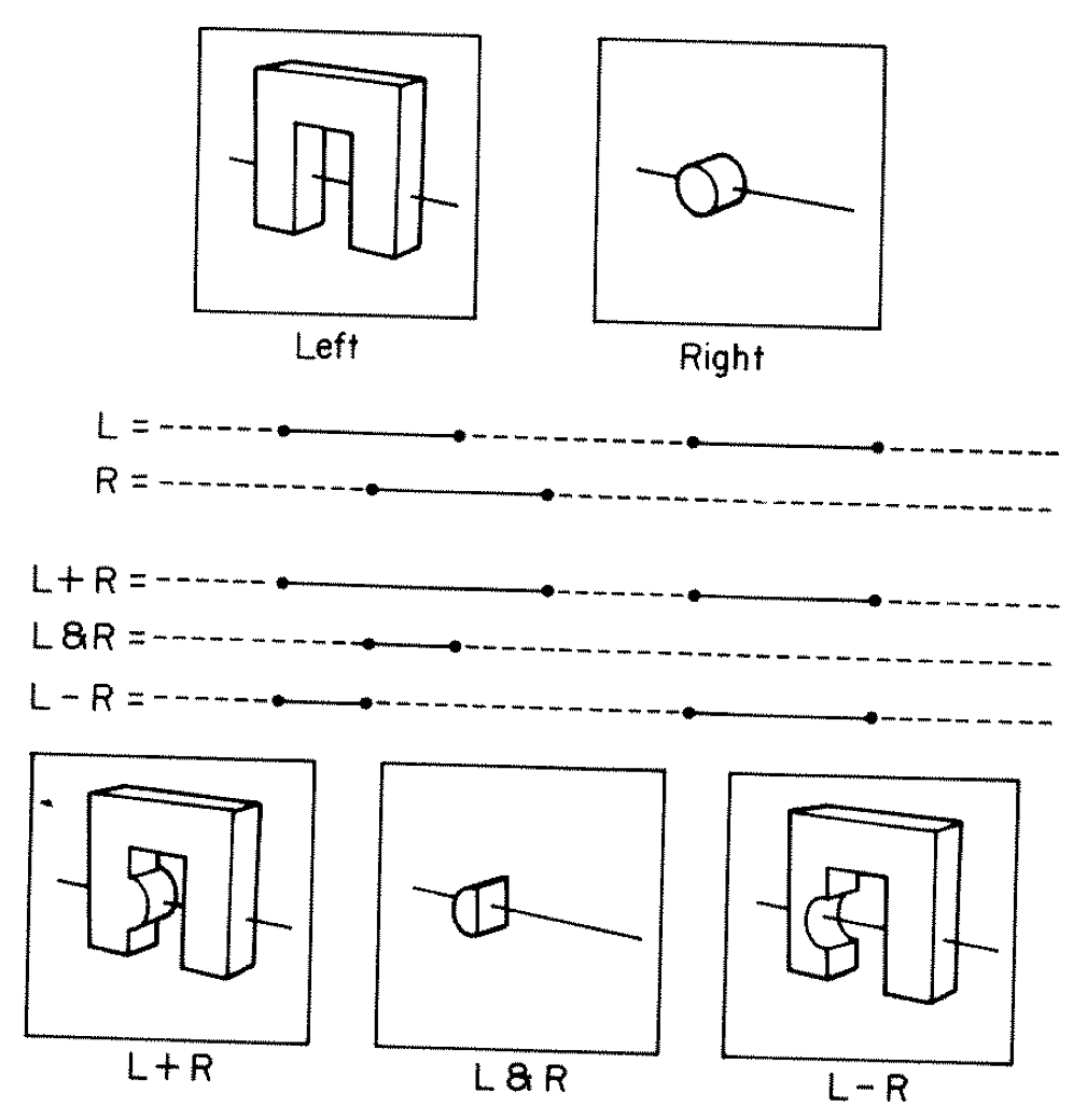
Classical Roth diagram approach
- find all ray/primitive intersects
- recursively combine inside intervals using CSG operator
- works from leaves upwards
Computational requirements:
- find all intersects, store them, order them
- recursive traverse
BUT : High performance on GPU requires:
- massive parallelism -> more the merrier
- low register usage -> keep it simple
- small stack size -> avoid recursion
Classical approach not appropriate on GPU
Ray intersection with general CSG binary trees, on GPU
Outside/Inside Unions
dot(normal,rayDir) -> Enter/Exit
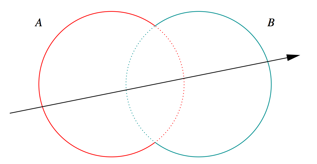
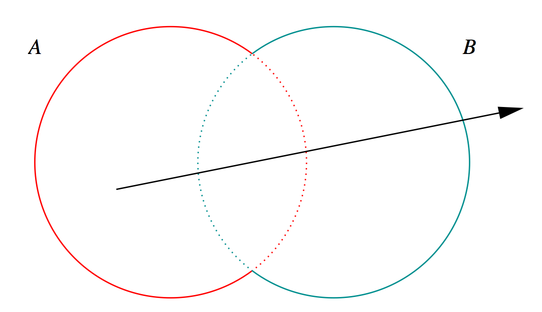
- A + B boundary not inside other
- A * B boundary inside other
Pick between pairs of nearest intersects, eg:
| UNION tA < tB | Enter B | Exit B | Miss B |
|---|---|---|---|
| Enter A | ReturnA | LoopA | ReturnA |
| Exit A | ReturnA | ReturnB | ReturnA |
| Miss A | ReturnB | ReturnB | ReturnMiss |
- Nearest hit intersect algorithm [1] avoids state
- sometimes Loop : advance t_min , re-intersect both
- classification shows if inside/outside
- Evaluative [2] implementation emulates recursion:
- recursion not allowed in OptiX intersect programs
- bit twiddle traversal of complete binary tree
- stacks of postorder slices and intersects
- Identical geometry to Geant4
- solving the same polynomials
- near perfect intersection match
- [1] Ray Tracing CSG Objects Using Single Hit Intersections, Andrew Kensler (2006)
- with corrections by author of XRT Raytracer http://xrt.wikidot.com/doc:csg
- [2] https://bitbucket.org/simoncblyth/opticks/src/tip/optixrap/cu/csg_intersect_boolean.h
- Similar to binary expression tree evaluation using postorder traverse.
CSG Complete Binary Tree Serialization -> simplifies GPU side
Bit Twiddling Navigation
- parent(i) = i/2 = i >> 1
- leftchild(i) = 2*i = i << 1
- rightchild(i) = 2*i + 1 = (i << 1) + 1
- leftmost(height) = 1 << height
Geant4 solid -> CSG binary tree (leaf primitives, non-leaf operators, 4x4 transforms on any node)
Serialize to complete binary tree buffer:
- no need to deserialize, no child/parent pointers
- bit twiddling navigation avoids recursion
- simple approach profits from small size of binary trees
- BUT: very inefficient when unbalanced
Height 3 complete binary tree with level order indices:
                                                   depth     elevation

                     1                               0           3

          10                   11                    1           2

     100       101        110        111             2           1

 1000 1001  1010 1011  1100 1101  1110  1111         3           0
postorder_next(i,elevation) = i & 1 ? i >> 1 : (i << elevation) + (1 << elevation) ; // from pattern of bits
Postorder tree traverse visits all nodes, starting from leftmost, such that children are visited prior to their parents.
Evaluative CSG intersection Pseudocode : recursion emulated
fullTree = PACK( 1 << height, 1 >> 1 )  // leftmost, parent_of_root(=0)
tranche.push(fullTree, ray.tmin)

while (!tranche.empty)         // stack of begin/end indices
{
    begin, end, tmin <- tranche.pop  ; node <- begin ;
    while( node != end )                   // over tranche of postorder traversal
    {
        elevation = height - TREE_DEPTH(node) ;
        if(is_primitive(node)){ isect <- intersect_primitive(node, tmin) ;  csg.push(isect) }
        else{
            i_left, i_right = csg.pop, csg.pop            // csg stack of intersect normals, t
            l_state = CLASSIFY(i_left, ray.direction, tmin)
            r_state = CLASSIFY(i_right, ray.direction, tmin)
            action = LUT(operator(node), leftIsCloser)(l_state, r_state)

            if(      action is ReturnLeft/Right)     csg.push(i_left or i_right)
            else if( action is LoopLeft/Right)
            {
                left = 2*node ; right = 2*node + 1 ;
                endTranche = PACK( node,  end );
                leftTranche = PACK(  left << (elevation-1), right << (elevation-1) )
                rightTranche = PACK(  right << (elevation-1),  node  )
                loopTranche = action ? leftTranche : rightTranche

                tranche.push(endTranche, tmin)
                tranche.push(loopTranche, tminAdvanced )  // subtree re-traversal with changed tmin
                break ; // to next tranche
            }
        }
        node <- postorder_next(node, elevation)         // bit twiddling postorder
    }
}
isect = csg.pop();         // winning intersect
https://bitbucket.org/simoncblyth/opticks/src/tip/optixrap/cu/csg_intersect_boolean.h
CSG Deep Tree : JUNO "fastener"

CSG Deep Tree : height 11 before balancing, too deep for GPU raytrace
 NTreeAnalyse height 11 count 25    ( un : union,  cy : cylinder, di : difference )
                                                                                       un

                                                                               un              di

                                                                       un          cy      cy      cy

                                                               un          cy

                                                       un          cy

                                               un          cy

                                       un          cy

                               un          cy

                       un          cy

               un          cy

       di          cy

   cy      cy
CSG trees are non-unique
- many possible expressions of same shape
- some much more efficiently represented as complete binary trees
CSG Deep Tree : Positivize tree using De Morgans laws
Positive form CSG Trees
Apply deMorgan pushing negations down tree
- A - B -> A * !B
- !(A*B) -> !A + !B
- !(A+B) -> !A * !B
- !(A - B) -> !(A*!B) -> !A + B
End with only UNION, INTERSECT operators, and some complemented leaves.
COMMUTATIVE -> easily rearranged
1st step to allow balancing : Positivize : remove CSG difference di operators
                                                     ...    ...

                                               un          cy

                                       un          cy

                               un          cy

                       un          cy

               un          cy

       di          cy

   cy      cy
                                                     ...    ...

                                               un          cy

                                       un          cy

                               un          cy

                       un          cy

               un          cy

       in          cy

   cy      !cy
CSG Deep Tree : height 4 after balancing, OK for GPU raytrace
NTreeAnalyse height 4 count 25
                                                               un

                               un                                                      un

               un                              un                      un                      in

       un              un              un              un          cy          in          cy     !cy

   cy      cy      cy      cy      cy      cy      cy      cy              cy     !cy
un : union, in : intersect, cy : cylinder, !cy : complemented cylinder
Balancing positive tree:
- classify tree operators and their placement
- mono-operator trees can easily be rearranged as union un and intersection in operators are commutative
- mono-operator above bileaf level can also easily be rearranged as the bileaf can be split off and combined
- create complete binary tree of appropriate size filled with placeholders
- populate the tree replacing placeholders
- prune (pull primitives up to avoid placeholder pairings)
Not a general balancer : but succeeds with all CSG solid trees from Daya Bay and JUNO so far
https://bitbucket.org/simoncblyth/opticks/src/default/npy/NTreeBalance.cpp
Opticks Analytic Daya Bay Near Site, GPU Raytrace (3)
Opticks Analytic Daya Bay Near Site, GPU Raytrace (1)
Opticks Analytic Daya Bay Near Site, GPU Raytrace (0)
Opticks Analytic Daya Bay Near Site, GPU Raytrace (2)
Opticks Analytic JUNO Chimney, GPU Raytrace (0)
Opticks Analytic JUNO PMT Snap, GPU Raytrace (1)
j1808_top_ogl
j1808_top_rtx
j1808_escapes
CSG : (Cylinder - Torus) PMT neck : spurious intersects
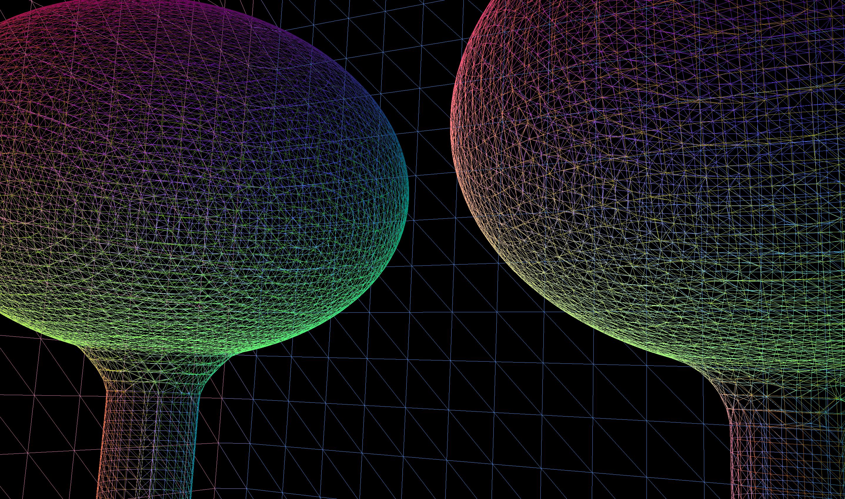
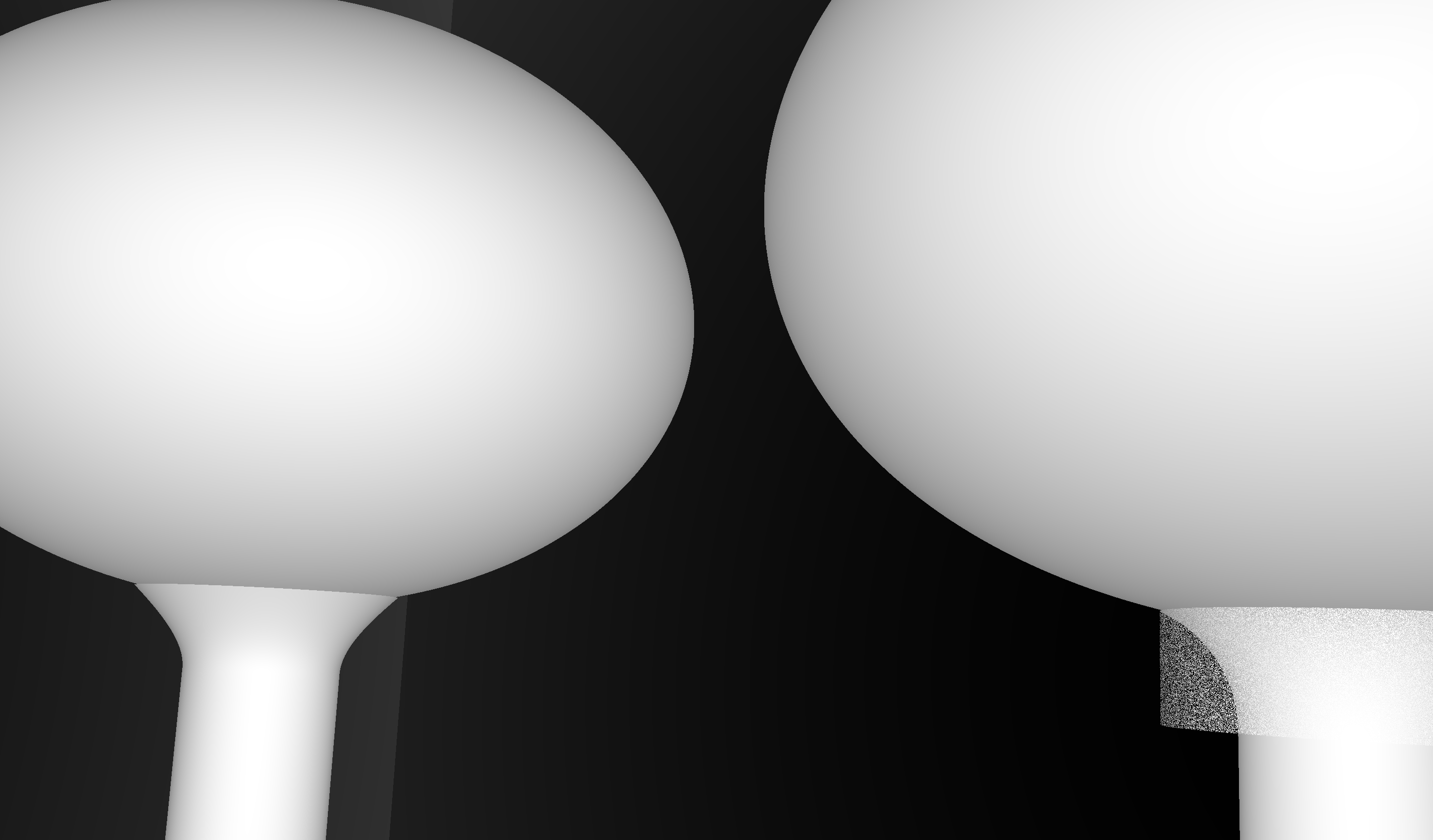
OptiX Raytrace and OpenGL rasterized wireframe comparing neck models:
- Ellipsoid + Hyperboloid + Cylinder
- Ellipsoid + (Cylinder - Torus) + Cylinder
Best Solution : use simpler neck model for physically unimportant PMT neck
CSG : Alternative PMT neck designs
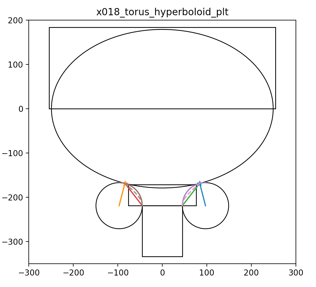
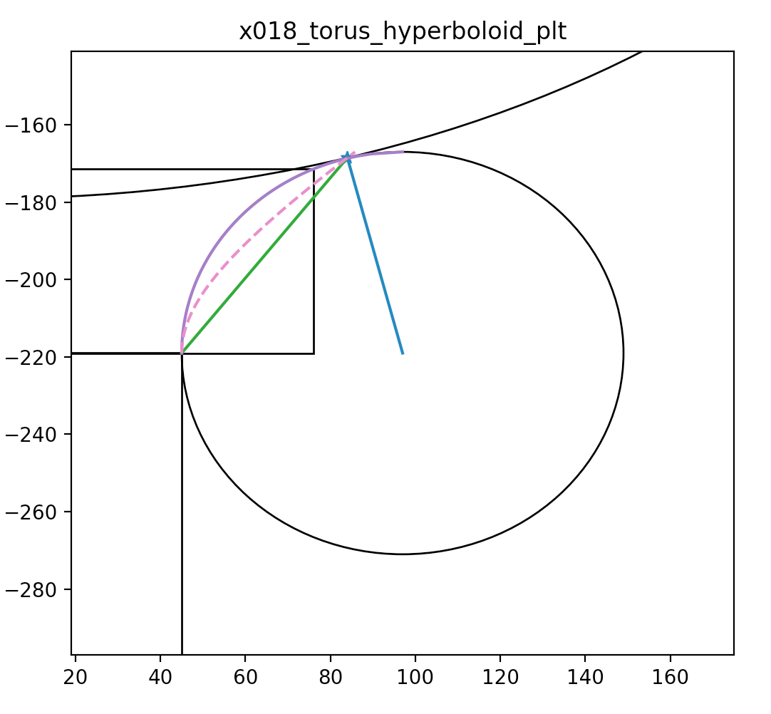
Hyperboloid and Cone defined using closest point on ellipse to center of torus circle
- Cylinder-Torus : purple line, Cone : green, simplest
- Hyperboloid : dashed magenta, works with Opticks, BUT G4Hype has no z-range flexibility
https://bitbucket.org/simoncblyth/opticks/src/tip/ana/x018_torus_hyperboloid_plt.py
Opticks : Auto-Instancing
Structure Tree Analysis
- structure node progeny digests
- sub-tree transforms & shapes
- instancing criteria
- number of repeats
- number of vertices
- exclude contained repeats
-> all repeated volumes + transforms
For JUNO, auto-finds:
- 20 inch PMTs, 3 inch PMTs
- acrylic fasteners, top-tracker elements
Avoids geometry specific code
OpenGL/OptiX instancing
- one definition of repeated geometry
- 4x4 transform for each placement
- drastic reduction in GPU memory
Opticks : translates G4 geometry to GPU, without approximation
Volumes -> Boundaries
Ray tracing favors Boundaries
Material/surface boundary : 4 indices
- outer material (parent)
- outer surface (inward photons, parent -> self)
- inner surface (outward photons, self -> parent)
- inner material (self)
Primitives labelled with unique boundary index
- ray primitive intersection -> boundary index
- texture lookup -> material/surface properties
- Direct Geometry : Geant4 "World" -> Opticks CSG -> GPU
- simpler : no G4DAE+GDML export/import
- Material/Surface/Scintillator properties
- interpolated to standard wavelength domain
- interleaved into "boundary" texture
- "reemission" texture for wavelength generation
- Structure
- repeated geometry instances identified (progeny digests)
- instance transforms used in OptiX/OpenGL geometry
- merge CSG trees into global + instance buffers
- export meshes to glTF 2.0 for 3D visualization
- Ease of Use
- easy geometry : just handover "World"
- easy config : modern CMake + BCM[1]
- ~easy event : modify G4Cerenkov + G4Scintillation
[1] Boost CMake 3.5+ modules : configure direct dependencies only
Opticks Export of G4 geometry to glTF 2.0
Emerging 3D Standard
"JPEG" of 3D

- Growing Adoption
- https://github.com/KhronosGroup/glTF https://www.khronos.org/gltf/
- <-- eg:Metal Renderer from GLTFKit
- https://github.com/warrenm/GLTFKit
- Similar to Opticks geocache
- JSON + binary buffers (eg NPY)
Opticks : translates G4 optical physics to GPU
GPU Resident Photons
- Seeded on GPU
- associate photons -> gensteps (via seed buffer)
- Generated on GPU, using genstep param:
- number of photons to generate
- start/end position of step
- Propagated on GPU
- Only photons hitting PMTs copied to CPU
Thrust: high level C++ access to CUDA

OptiX : single-ray programming model -> line-by-line translation
- CUDA Ports of Geant4 classes
- G4Cerenkov (only generation loop)
- G4Scintillation (only generation loop)
- G4OpAbsorption
- G4OpRayleigh
- G4OpBoundaryProcess (only a few surface types)
- Modify Cerenkov + Scintillation Processes
- collect genstep, copy to GPU for generation
- avoids copying millions of photons to GPU
- Scintillator Reemission
- fraction of bulk absorbed "reborn" within same thread
- wavelength generated by reemission texture lookup
- Opticks (OptiX/Thrust GPU interoperation)
- OptiX : upload gensteps
- Thrust : seeding, distribute genstep indices to photons
- OptiX : launch photon generation and propagation
- Thrust : pullback photons that hit PMTs
- Thrust : index photon step sequences (optional)
Validation : Compare Opticks/Geant4 with Simple Lights/Geometries
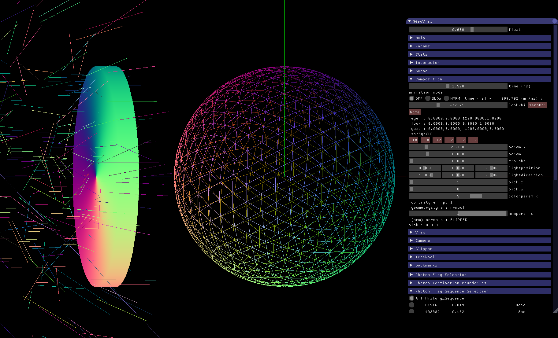
1M Photons -> Water Sphere (S-Polarized)
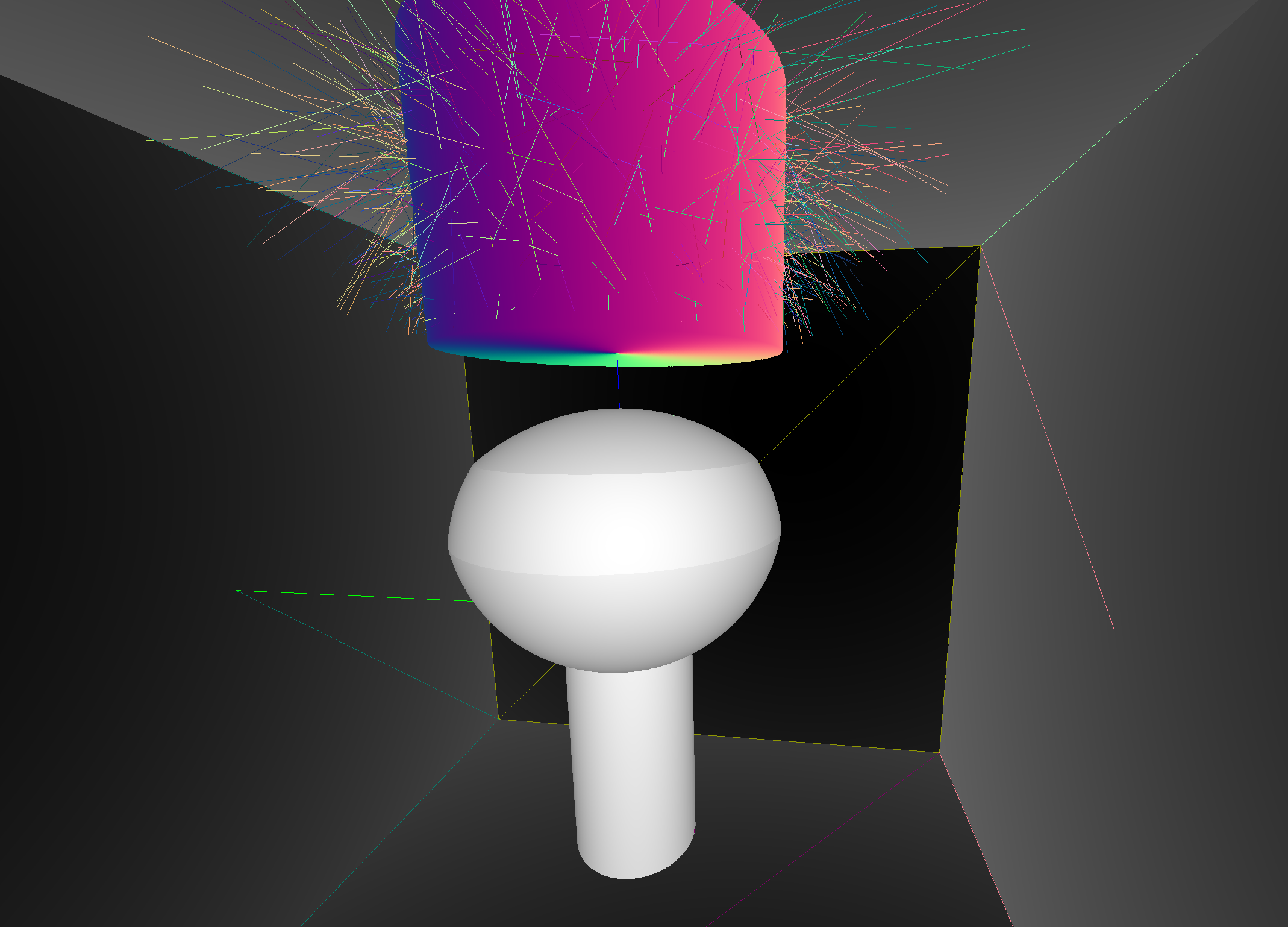
0.5M Photons -> Dayabay PMT

- Photon step records
- 128 bit per step : highly compressed position, time, wavelength, polarization vector, material/history codes
- Photon flag sequence
- 16x 4-bit step flags recorded in uint64 sequence, indexed using Thrust GPU sort (1M indexed ~0.040s)
- Final Photons
- Uncompressed : position, time, wavelength, direction, polarization, flags
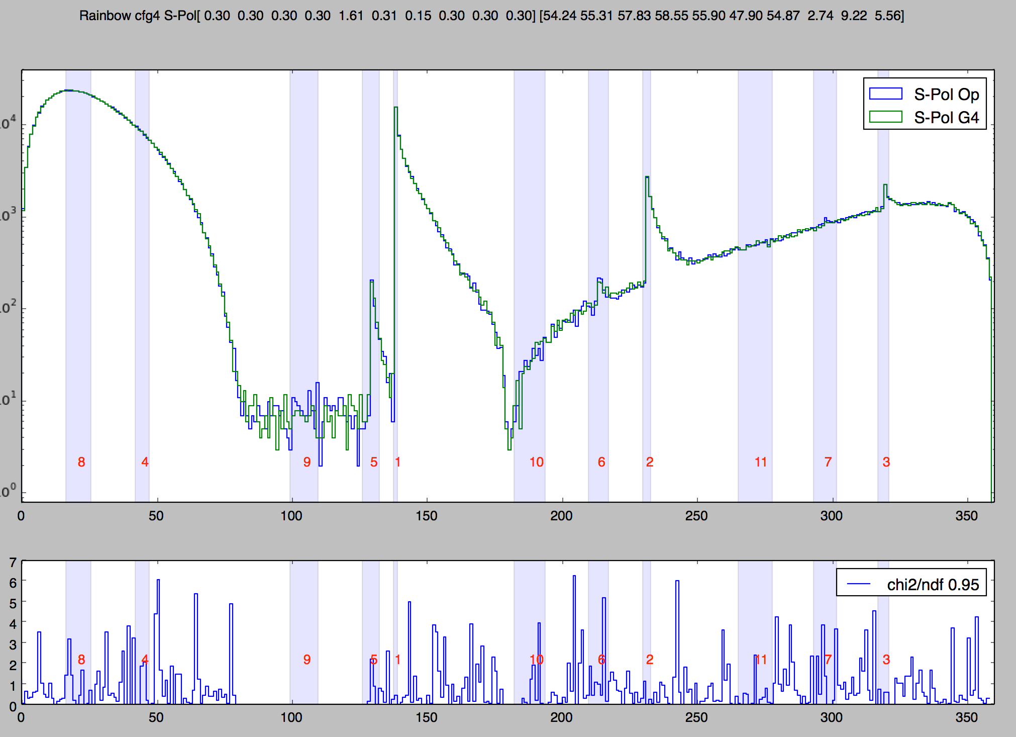
1M Rainbow S-Polarized, Comparison Opticks/Geant4
Deviation angle(degrees) of 1M parallel monochromatic photons in disc shaped beam incident on water sphere. Numbered bands are visible range expectations of first 11 rainbows. S-Polarized intersection (E field perpendicular to plane of incidence) arranged by directing polarization radially.
Take Control of Geant4 Random Number Generator (RNG)
- controlling Geant4 randoms -> can align CPU and GPU sequences -> directly matched simulations
- need separate sequences for each photon : parallel GPU processing means order is undefined
After CAlignEngine::SetSequenceIndex(int index) : subsequent G4UniformRand() give randoms from sequence index
// EngineMinimalTest.cc : demonstrate G4UniformRand control
##include "Randomize.hh"                                              $ EngineMinimalTest
                                                                     0.13049
struct MyEngine : public CLHEP::MixMaxRng  // MixMax is default      0.617751
{                                                                    0.995947
    double flat(){ return .42 ; }                                    0.495902
};                                                                   0.112917
                                                                     0.289871
int main(int argc, char** argv)                                      0.473044
{                                                                    0.837619
    if(argc > 1)                                                     0.359356
       CLHEP::HepRandom::setTheEngine(new MyEngine());               0.926938

    for( int i=0 ; i < 10 ; i++)                                     $ EngineMinimalTest 1
         std::cout << G4UniformRand() << std::endl ;                 0.42
                                                                     0.42
    return 0 ;                                                       0.42
}                                                                    ...
https://bitbucket.org/simoncblyth/opticks/src/default/cfg4/CAlignEngine.cc
Validation : Aligning CPU and GPU Simulations
lldb python scripting
- access C++ program state from python
- step-by-step compare photon parameters with expectations, break at deviations
Auto-configure breakpoints using code markers:
opticks/tools/autobreakpoint.py opticks/tools/g4lldb.py
Ubiquitous Data access with NPY
All Opticks data managed in NumPy buffers, easy access from python,C++,CUDA,lldb-python
Aligned zipping together of code and RNG values
- common input photon sample generated on CPU
- random number sequences generated on GPU (cuRAND) and persisted to file (NPY buffers)
Single executable lldb OKG4Test:
- run Opticks GPU simulation, persist event
- run Geant4 simulation
- step-by-step check each G4 photon follows Opticks history and parameters, break at deviations
- fix cause of misaligned RNG consumption, or other deviation
- tricks needed on both sides : burning RNGs, jump backs
Payoff : simplest possible direct comparison validation
http://bitbucket.com/simoncblyth/opticks/src/tip/tools/autobreakpoint.py
(lldb) help breakpoint command add
Validation : Direct comparison of GPU/CPU NumPy arrays
CPU/GPU matching
- Simple geometries
- same geometry, same physics, same results
- Full geometries
- aligned running will find geometry issues eg coincident surface ambiguity
- NEXT:
- align generation, reemission, more geometries
tboolean-box simple geometry test
- 100k photons : position, time, polarization : 1.2M floats
- 34 deviations > 1e-4 (mm or ns), largest 4e-4
- deviants all involve scattering (more flops?)
In [11]: pdv = np.where(dv > 0.0001)[0]
In [12]: ab.dumpline(pdv)
      0   1230 : TO BR SC BT BR BT SA
      1   2413 : TO BT BT SC BT BR BR BT SA
      2   9041 : TO BT SC BR BR BR BR BT SA
      3  14510 : TO SC BT BR BR BT SA
      4  14747 : TO BT SC BR BR BR BR BR BR BR
      5  14747 : TO BT SC BR BR BR BR BR BR BR
    ...

In [20]: ab.b.ox[pdv,0]                                 In [21]: ab.a.ox[pdv,0]
Out[20]:                                                Out[21]:
A()sliced                                               A()sliced
A([    [-191.6262, -240.3634,  450.    ,    5.566 ],    A([    [-191.626 , -240.3634,  450.    ,    5.566 ],
       [ 185.7708, -133.8457,  450.    ,    7.3141],           [ 185.7708, -133.8456,  450.    ,    7.3141],
       [-450.    , -104.4142,  311.143 ,    9.0581],           [-450.    , -104.4142,  311.1431,    9.0581],
       [  83.6955,  208.9171, -450.    ,    5.6188],           [  83.6954,  208.9172, -450.    ,    5.6188],
       [  32.8972,  150.    ,   24.9922,    7.6757],           [  32.8973,  150.    ,   24.992 ,    7.6757],
       [  32.8972,  150.    ,   24.9922,    7.6757],           [  32.8973,  150.    ,   24.992 ,    7.6757],
       [ 450.    , -186.7449,  310.6051,    5.0707],           [ 450.    , -186.7451,  310.605 ,    5.0707],
       [ 299.2227,  318.1443, -450.    ,    4.8717],           [ 299.2229,  318.144 , -450.    ,    4.8717],
 ...
Coincident Faces are Primary Cause of Issues : Spurious Intersects
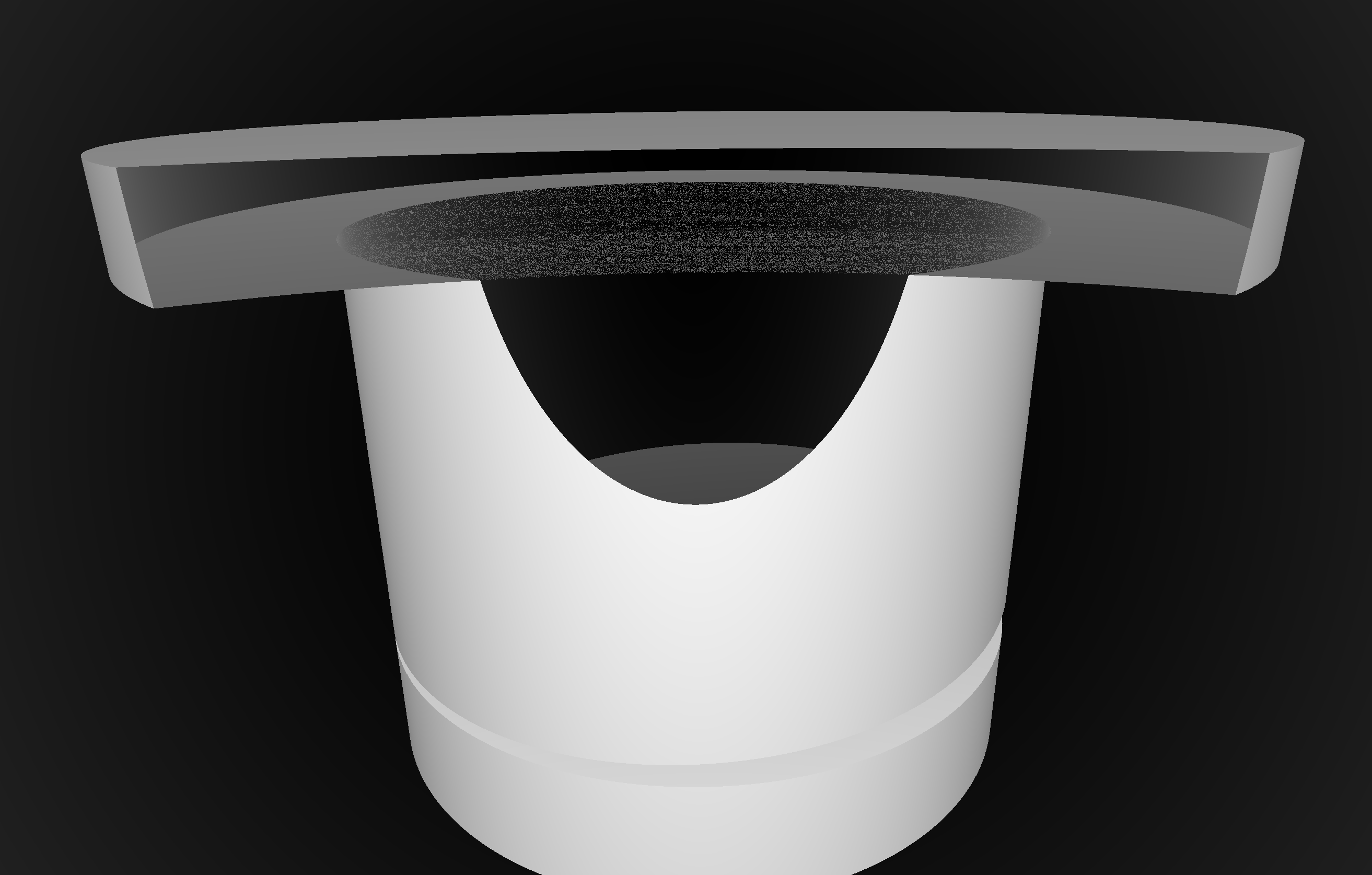
Cylinder - Cone
Coincident endcaps -> spurious intersects
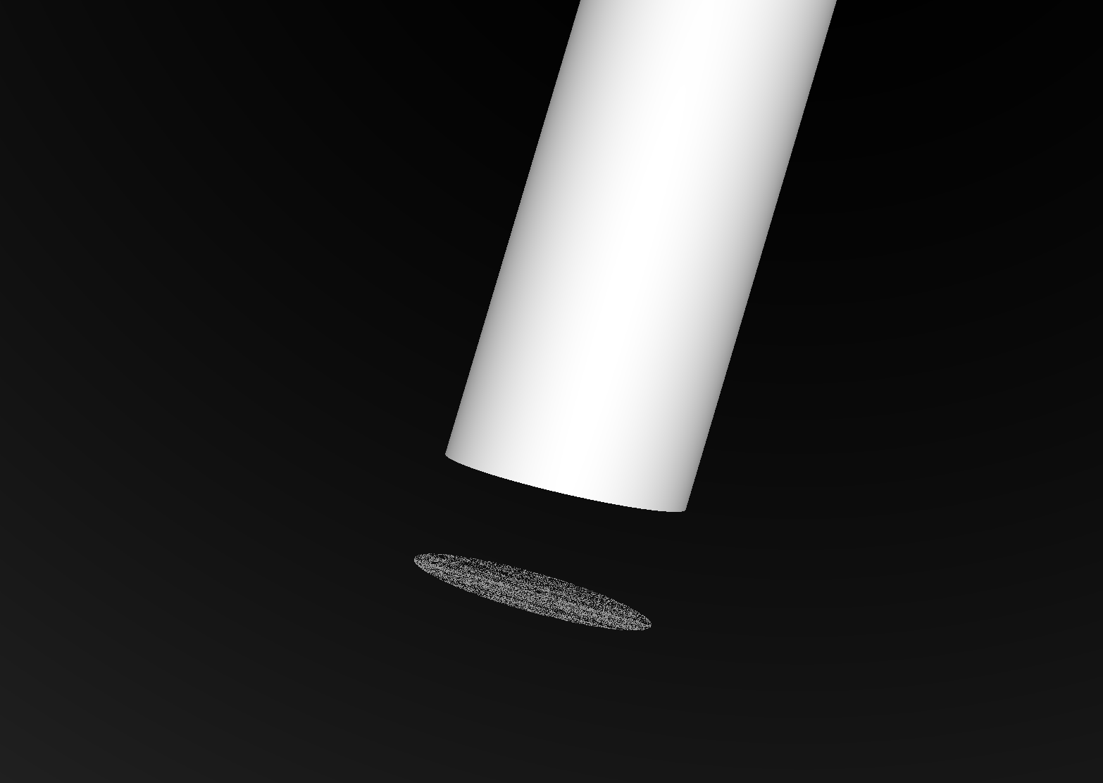
Grow subtracted cone downwards, avoids coincidence : does not change composite solid
Coincidences common (alignment too tempting?). To fix:
- A-B : grow correct dimension of subtracted shape
- A+B : grow smaller interface shape into bigger, making join
- case-by-case fixes straightforward, not so easy to automate
- WIP: automated coincidence finder/fixer
Summary
Highlights
- identical GPU geometry, auto-translated
- aligned running -> simple validation
- expect: Opticks > 1000x Geant4 (with workstation GPUs)
- more photons -> more overall speedup
- 99% -> 100x

Opticks enables Geant4 based simulations to benefit from effectively zero time and zero CPU memory optical photon simulation, due to massive parallelism made accessible by NVIDIA OptiX.

- Drastic speedup -> better detector understanding -> greater precision
- Performance discontinuity -> new possibilities -> imagination required

Subscribe to stay informed on Opticks:
Opticks References
Introductions
- https://bitbucket.org/simoncblyth/intro_to_numpy
- Introducing NumPy, Array-oriented computing
- https://bitbucket.org/simoncblyth/intro_to_cuda
- Introducing CUDA and Thrust
- https://github.com/simoncblyth/np
- NumPy Array Serialization from C++
- https://simoncblyth.bitbucket.io
- Opticks presentations and videos
- https://groups.io/g/opticks
- Opticks mailing list archive
- opticks+subscribe@groups.io
- send email to this address, to subscribe
- https://simoncblyth.bitbucket.io/opticks/index.html
- Opticks installation instructions
- https://bitbucket.org/simoncblyth/opticks
- Opticks code repository
OpticksDocs
Open Source Opticks
Documentation, install instructions. Repository.
- Mac, Linux, Windows (*)
- ~20 C++ projects, ordered by dependency
- ~370 "Unit" Tests (CMake/CTest)
- ~50 integration tests: tpmt, trainbow, tprism, treflect, tlens, tnewton, tg4gun, ...
- NumPy/Python analysis/debugging scripts
Geometry/event data use NumPy serialization:
import numpy as np
a = np.load("photons.npy")
(*) Windows VS2015, non-CUDA only, not recently!
The Zen of Numpy, by its creator, Travis Oliphant
Strided is better than scattered.
Contiguous is better than strided.
Descriptive is better than imperative[1] (e.g. data-types).
Array-orientated is better than object-oriented.
Broadcasting is a great idea -- use where possible!
Vectorized is better than an explicit loop.
Unless its complicated -- then use Cython or numexpr.
Think in higher dimensions.
My take : best tool depends on nature of data
- NumPy shines for large[2] and simple data ; splitting data to make it simple brings other benefits !
- NumPy holistic approach : prepares you for vectorized and parallel processing
- no-looping makes for an terse, intuitive interactive interface
[1] imperative means step by step how to do something
[2] but not so large that has trouble fitting in memory, np.memmap is possible but better to avoid for simplicity
NPY minimal file format : metadata header + data buffer : trivial to parse
- data accessible from anywhere : C/C++/CUDA/python/... ; Simple to memcpy() or cudaMemcpy() to GPU
In [1]: a = np.arange(10)        # array of 10 ints : 64 bit, 8 bytes each
In [2]: np.save("a.npy", a )       # persist the array : serializing it into a file

In [3]: a2 = np.load("a.npy")         # load array from file into memory
In [4]: assert np.all( a == a2 )      # check all elements the same

In [5]: !xxd a.npy                   # run xxd in shell to hexdump the byte contents of the file

00000000: 934e 554d 5059 0100 7600 7b27 6465 7363  .NUMPY..v.{ desc
00000010: 7227 3a20 273c 6938 272c 2027 666f 7274  r': '<i8', 'fort
00000020: 7261 6e5f 6f72 6465 7227 3a20 4661 6c73  ran_order : Fals
00000030: 652c 2027 7368 6170 6527 3a20 2831 302c  e, 'shape': (10,    # minimal metadata : type, shape
00000040: 292c 207d 2020 2020 2020 2020 2020 2020  ), }
00000050: 2020 2020 2020 2020 2020 2020 2020 2020
00000060: 2020 2020 2020 2020 2020 2020 2020 2020
00000070: 2020 2020 2020 2020 2020 2020 2020 200a                 .    # 128 bytes of header
00000080: 0000 0000 0000 0000 0100 0000 0000 0000  ................
00000090: 0200 0000 0000 0000 0300 0000 0000 0000  ................
000000a0: 0400 0000 0000 0000 0500 0000 0000 0000  ................    # data buffer
000000b0: 0600 0000 0000 0000 0700 0000 0000 0000  ................
000000c0: 0800 0000 0000 0000 0900 0000 0000 0000  ................

In [6]: !ls -l a.npy     # small 128 byte header + (8 bytes per integer)*10 = 208 bytes total
-rw-r--r--  1 blyth  staff  208 Sep 13 11:01 a.npy

In [7]: a
Out[7]: array([0, 1, 2, 3, 4, 5, 6, 7, 8, 9])
In [8]: a.shape
Out[8]: (10,)
One possibility for compression with blosc http://bcolz.blosc.org/en/latest/intro.html
