Opticks : GPU Optical Photon Simulation for Particle Physics with NVIDIA OptiX

Opticks: GPU photon simulation via NVIDIA OptiX ;

Applied to neutrino telescope simulations ?

Opticks : GPU Optical Photon Simulation for Particle Physics with NVIDIA OptiX Talk

Opticks is an open source project that applies state-of-the-art GPU ray tracing from NVIDIA OptiX to optical photon simulation and integrates this with Geant4. This results in drastic speedups of more than 1500 times single threaded Geant4.

Any simulation limited by optical photons can remove those limits by using Opticks.

This render shows the photons resulting from a muon crossing the JUNO scintillator, each line represents a single photon.

The number of photons across track lengths up to 35m in the scintillator is about 70M

Outline Opticks

• Context and Problem
  • Jiangmen Underground Neutrino Observatory (JUNO)
  • Optical Photon Simulation Problem...
• Tools to create Solution
  • Optical Photon Simulation ≈ Ray Traced Image Rendering
  • Rasterization and Ray tracing
  • Turing Built for RTX
  • BVH : Bounding Volume Hierarchy
  • NVIDIA OptiX Ray Tracing Engine
• Opticks : The Solution
  • Geant4 + Opticks Hybrid Workflow : External Optical Photon Simulation
  • Opticks : Translates G4 Optical Physics to CUDA/OptiX
  • Opticks : Translates G4 Geometry to GPU, Without Approximation
  • CUDA/OptiX Intersection Functions for ~10 Primitives
  • CUDA/OptiX Intersection Functions for Arbitrarily Complex CSG Shapes
• Validation and Performance
  • Random Aligned Bi-Simulation -> Direct Array Comparison
  • Perfomance Scanning from 1M to 400M Photons
• Overview + Links

Outline Opticks Talk

This will be a talk of two halves:

• first I will introduce Opticks and how it solves the problem of optical photon simulation for JUNO

Outline of Graphics/GPU background + Application to neutrino telescopes

• GPU + Parallel Processing Background
  • Amdahls "Law" : Expected speedup limited by serial processing
  • Understanding GPU Graphical Origins -> Effective GPU Computation
  • CPU Optimizes Latency, GPU Optimizes Throughput
  • How to make effective use of GPUs ? Parallel/Simple/Uncoupled
  • GPU Demands Simplicity (Arrays) -> Big Benefits : NumPy + CuPy
  • Survey of High Level General Purpose CUDA Packages
• Graphics History/Background
  • 50 years of rendering progress
  • 2018 : NVIDIA RTX : Project Sol Demo
  • Monte Carlo Path Tracing in Movie Production
  • Fundamental "Rendering Equation" of Computer Graphics
  • Neumann Series solution of Rendering Equation
  • Noise : Problem with Monte Carlo Path Tracing
  • NVIDIA OptiX Denoiser
  • Physically Based Rendering Book : Free Online
  • Optical Simulations : Graphics vs Physics
• Neutrino Telescope Optical simulations
  • Giga-photon propagations : Re-usable photon "snapshots"
  • Opticks Rayleigh Scattering : CUDA line-by-line port of G4OpRayleigh
  • Developing a photon "snapshot" cache
  • Photon Mapping
• Summary

Outline of Graphics/GPU background + Application to neutrino telescopes Talk

• Then I will cover GPU and graphics backgrounds which can help to handle really large propagation of billions of photons
• I will go into some details on computer graphics techniques as I think there is strong potential to re-purposing them to help physics simulations

JUNO_Intro_2

JUNO_Intro_2 Talk

JUNO will be the worlds largest liquid scintillator detector, with a spherical 20,000 ton volume of scintillator surrounded by a water pool buffer which also provides water cherenkov detection.

The scintillator is instrumented with 18 thousand 20-inch PMTs and 25 thousand 3-inch PMTs

JUNO_Intro_3

JUNO_Intro_3 Talk

JUNO will be able to detect neutrinos from many terrestrial and extra-terrestrial sources including : solar, atmospheric, geo-neutrinos.

Despite 700 m of overburden the largest backgrounds to these neutrino signals will be from cosmic muon induced processes.

A muon veto is used to control the backgrounds.

However to minimize the time and volume vetoed, it is necessary to have a good muon reconstruction which means that we need large samples of cosmic muons.

Geant4 : Monte Carlo Simulation Toolkit

Geant4 : Monte Carlo Simulation Toolkit Talk

Geant4 is the standard toolkit used to simulate detectors across several fields.

Geant4 : Monte Carlo Simulation Toolkit Generality

Geant4 : Monte Carlo Simulation Toolkit Generality Talk

Geant4 is a very general tool : but it is mostly not needed for the simulation of optical photons

Optical Photon Simulation Problem...

Optical Photon Simulation Problem... Talk

Muons travelling across the liquid scintillator will yield many tens of millions of optical photons. This is a huge memory and time challenge for Geant4 monte carlo production.

Most of the CPU time is taken finding intersections between photons and geometry Fortunately simulation is not alone in this bottleneck.

Optical photons are naturally parallel, with only Cherenkov and Scintillation production being relevant and we are only interested in photons collected at PMTs.

These characteristics make it straightforward to integrate an external optical simulation.

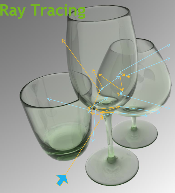
Optical Photon Simulation ≈ Ray Traced Image Rendering

Not a Photo, a Calculation

http://on-demand.gputechconf.com/siggraph/2013/presentation/SG3106-Building-Ray-Tracing-Applications-OptiX.pdf

Much in common : geometry, light sources, optical physics

• simulation : photon parameters at PMT detectors
• rendering : pixel values at image plane
• both limited by ray geometry intersection, aka ray tracing

Many Applications of ray tracing :

• advertising, design, architecture, films, games,...
• -> huge efforts to improve hw+sw over 30 yrs

Optical Photon Simulation ≈ Ray Traced Image Rendering Talk

Optical photon simulation and ray traced image rendering have a lot in common.

They are both limited by ray geometry intersection (or ray tracing)

With simulation you want to know photon parameters at PMTs, with rendering you need pixel values at the image plane.

Both these are limited by ray geometry intersection, which is also known as ray tracing.

Ray tracing is used across many industries, which means that are huge efforts across decades to improve ray tracing perfromance.

Ray-tracing vs Rasterization

Ray-tracing vs Rasterization Talk

It is good to clarify the difference between the two primary graphics rendering techniques

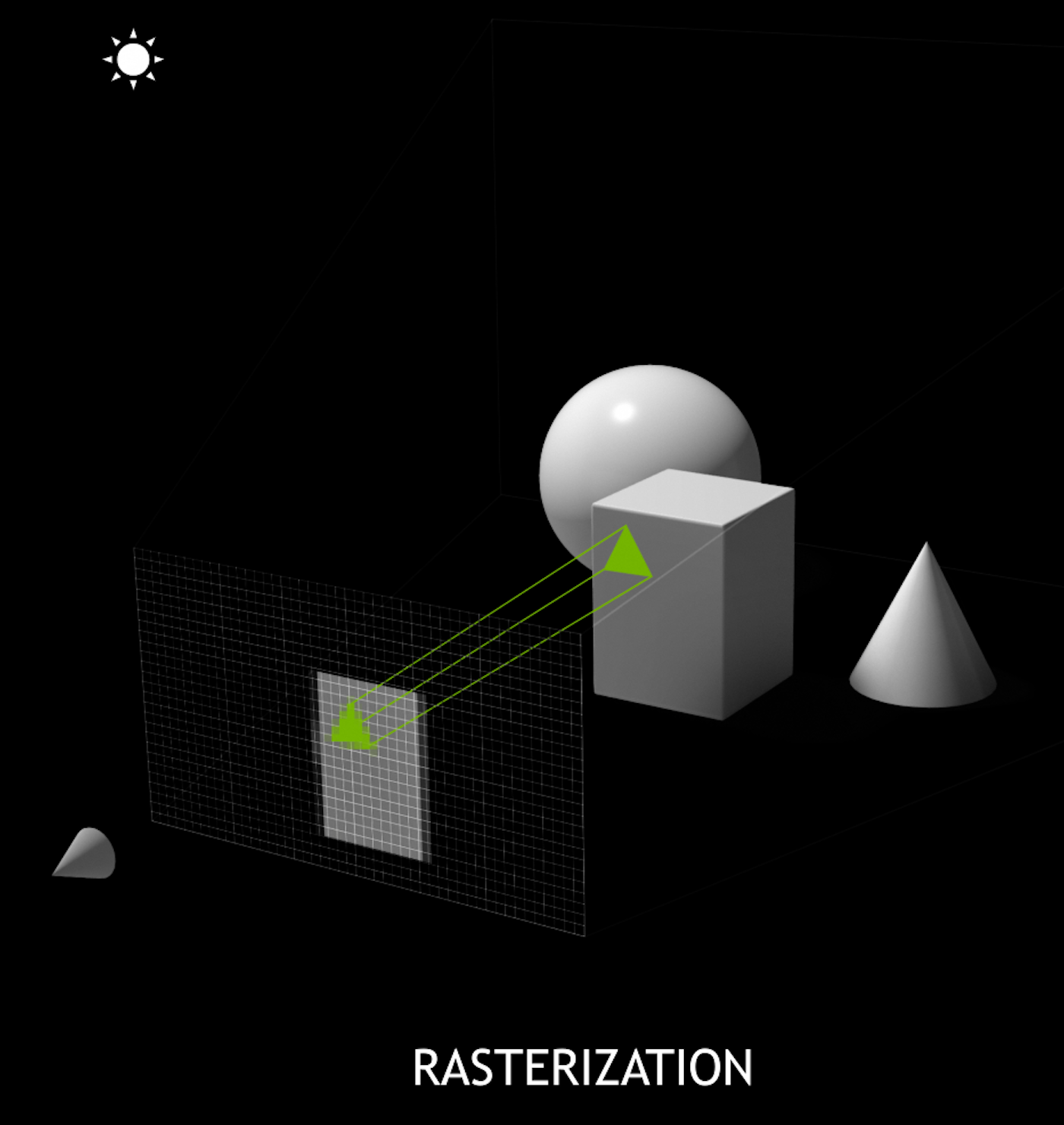
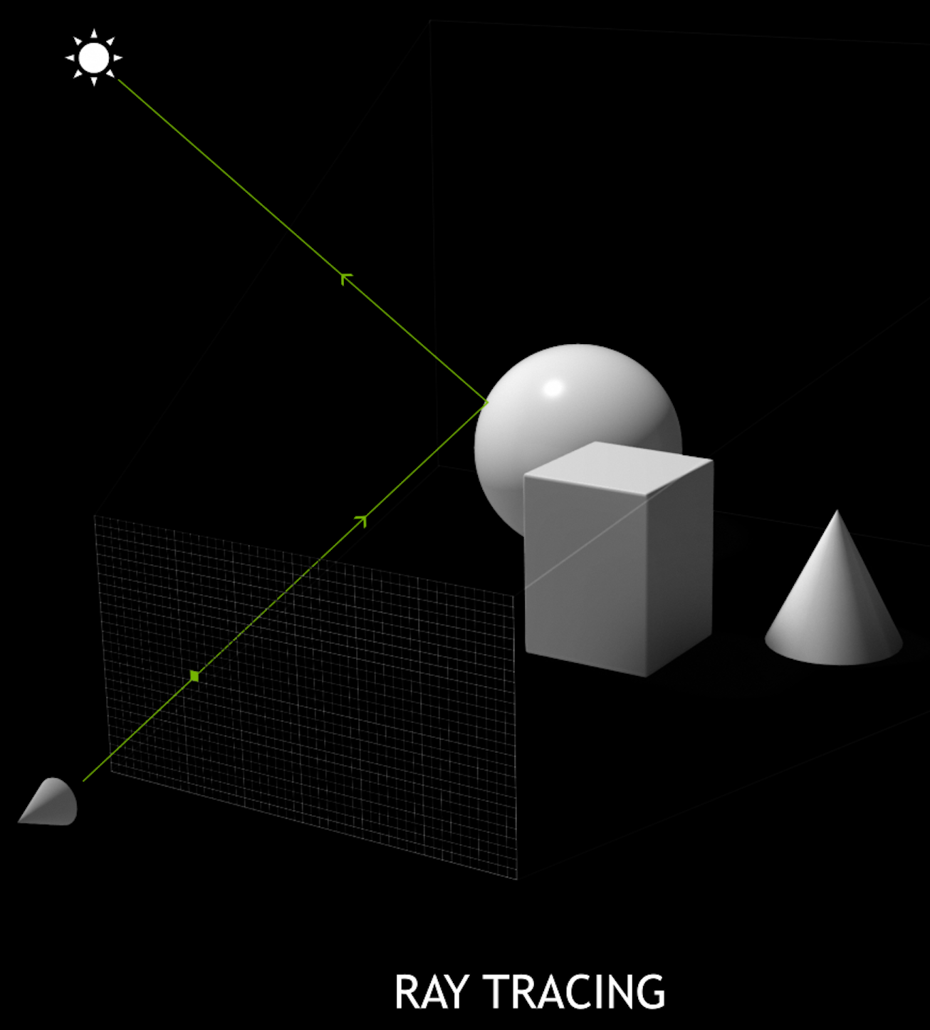
Rasterization is the most common rendering technique

• it starts from the objects in a scene, and projects them onto pixels in image plane
• this requires approximate triangulated geometry

Ray tracing

• starts from the pixels, casts rays out into the 3D scene and finds intersects
• this can use analytic geometry, without approximation (just like Geant4)
• its easier to create realistic images with ray tracing because it is closer to the physics

Ray tracing is an overloaded term. In some contexts it means just the ray transport from an origin to an intersection. But is also refers more generally to a specific rendering technique and even more generally a class of rendering techniques.

SIGGRAPH_2018_Announcing_Worlds_First_Ray_Tracing_GPU

SIGGRAPH_2018_Announcing_Worlds_First_Ray_Tracing_GPU Talk

Two years ago NVIDIA announced a leap in ray tracing performance with the Quadro RTX GPU : which it calls the worlds first ray tracing GPU As it has hardware dedicated to accelerating ray tracing.

NVIDIA claims it can reach 10 billion ray geometry intersections per second with a single GPU.

Assuming each simulated photon costs 10 rays, that means the upper limit per GPU is 1 billion photons/second.

TURING BUILT FOR RTX 2

TURING BUILT FOR RTX 2 Talk

The performance jump is done by offloading ray tracing from the general purpose SM (streaming multiprocessor) to the fixed function RT core, which frees up the SM.

NVIDIA RTX Metro Exodus

NVIDIA RTX Metro Exodus Talk

To gamers and movie makers these RTX GPUs enable:

• real-time cinematic rendering

RTX is hybrid rendering using:

• three types of dedicated hardware
• plus the general purpose SM, which runs the CUDA

Spatial Index Acceleration Structure

Spatial Index Acceleration Structure Talk

The principal technique to accelerate ray geometry intersection is an acceleration structure called a bounding volume hierarchy

This divides space into progressively smaller boxes which forms a spatial index.

Traversing the tree of bounds allows to minimize tests needed to find an intersect.

With some geometry it is possible for the traversal to be done on the dedicated RT cores.

NVIDIA® OptiX™ Ray Tracing Engine -- http://developer.nvidia.com/optix

OptiX Raytracing Pipeline

Analogous to OpenGL rasterization pipeline:

OptiX makes GPU ray tracing accessible

• accelerates ray-geometry intersections
• simple : single-ray programming model
• "...free to use within any application..."
• access RT Cores[1] with OptiX 6.0.0+ via RTX™ mode

NVIDIA expertise:

• ~linear scaling up to 4 GPUs
• acceleration structure creation + traversal (Blue)
• instanced sharing of geometry + acceleration structures
• compiler optimized for GPU ray tracing

Opticks provides (Yellow):

• ray generation program
• ray geometry intersection+bbox programs

[1] Turing RTX GPUs

NVIDIA® OptiX™ Ray Tracing Engine -- http://developer.nvidia.com/optix Talk

• NVIDIA OptiX is a CUDA interface to the NVIDIA BVH acceleration structure
• it is a ray tracing specific compiler

OptiX creates GPU kernels by compiling together:

• user programs for ray generation and geometry intersection (yellow boxes)
• with NVIDIA traversal programs (blue boxes)

most of Opticks on the GPU is in the ray generation and intersection programs

• OptiX accelerates the intersection...
• Triangle intersection can be done on the RT Cores,
• other shapes needs CUDA implementations, and runs on the SM

Geant4OpticksWorkflow

Geant4OpticksWorkflow Talk

SMALL So : how can an external optical photon simulation be integrated with Geant4 ?

In the standard workflow the Geant4 Scintillation and Cerenkov processes calculate a number of photons and then loop generating these and collecting them as secondaries

In the hybrid workflow, this generation is split between the CPU and GPU with "Gensteps" acting as the bridge. These Genstep parameters include the number of photons, positions and everything else needed in the generation loop.

The result is a very simple port of the generation loop to the GPU.

Its doubly helpful to generate photons on GPU, as then they take no CPU memory.

So can entirely offload photon memory to the GPU with only hits needing CPU memory.

Also this keeps the overheads low as gensteps are typically a factor of 100 smaller than photons.

The geometry is also needed on the GPU, with all material and surface properties.

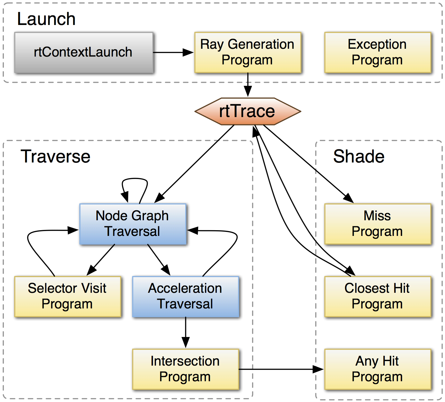
Opticks : Translates G4 Optical Physics to CUDA/OptiX

GPU Resident Photons

Seeded on GPU

associate photons -> gensteps (via seed buffer)

Generated on GPU, using genstep param:

• number of photons to generate
• start/end position of step

Propagated on GPU

Only photons hitting PMTs copied to CPU

Thrust: high level C++ access to CUDA

• https://developer.nvidia.com/Thrust

OptiX : single-ray programming model -> line-by-line translation

CUDA Ports of Geant4 classes

• G4Cerenkov (only generation loop)
• G4Scintillation (only generation loop)
• G4OpAbsorption
• G4OpRayleigh
• G4OpBoundaryProcess (only a few surface types)

Modify Cherenkov + Scintillation Processes

• collect genstep, copy to GPU for generation
• avoids copying millions of photons to GPU

Scintillator Reemission

• fraction of bulk absorbed "reborn" within same thread
• wavelength generated by reemission texture lookup

Opticks (OptiX/Thrust GPU interoperation)

• OptiX : upload gensteps
• Thrust : seeding, distribute genstep indices to photons
• OptiX : launch photon generation and propagation
• Thrust : pullback photons that hit PMTs
• Thrust : index photon step sequences (optional)

Opticks : Translates G4 Optical Physics to CUDA/OptiX Talk

This repeats what I just explained on the diagram

• essentially the necessary Geant4 optical physics is ported to CUDA
• the crucial thing to realize is that the photons are GPU resident
  • they are generated, propagated and visualized all in GPU buffers
  • only collected photons need to be copied to the CPU

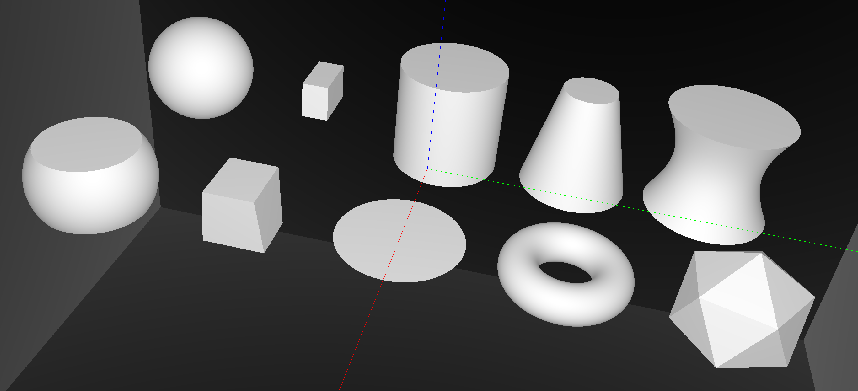
G4Solid -> CUDA Intersect Functions for ~10 Primitives

• 3D parametric ray : ray(x,y,z;t) = rayOrigin + t * rayDirection
• implicit equation of primitive : f(x,y,z) = 0
• -> polynomial in t , roots: t > t_min -> intersection positions + surface normals

Sphere, Cylinder, Disc, Cone, Convex Polyhedron, Hyperboloid, Torus, ...

G4Solid -> CUDA Intersect Functions for ~10 Primitives Talk

Geometry starts from primitive shapes.

NVIDIA OptiX doesnt provide primitives : My Opticks has ray geometry intersection for these shapes implemented with polynomial root finding.

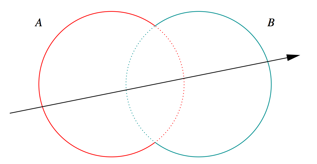
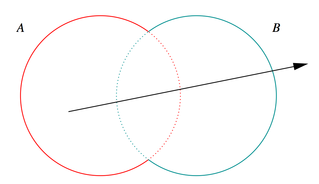
G4Boolean -> CUDA/OptiX Intersection Program Implementing CSG

Outside/Inside Unions

dot(normal,rayDir) -> Enter/Exit

• A + B boundary not inside other
• A * B boundary inside other

Complete Binary Tree, pick between pairs of nearest intersects:

• Nearest hit intersect algorithm [1] avoids state
  • sometimes Loop : advance t_min , re-intersect both
  • classification shows if inside/outside
• Evaluative [2] implementation emulates recursion:
  • recursion not allowed in OptiX intersect programs
  • bit twiddle traversal of complete binary tree
  • stacks of postorder slices and intersects
• Identical geometry to Geant4
  • solving the same polynomials
  • near perfect intersection match

[1] Ray Tracing CSG Objects Using Single Hit Intersections, Andrew Kensler (2006)

with corrections by author of XRT Raytracer http://xrt.wikidot.com/doc:csg

[2] https://bitbucket.org/simoncblyth/opticks/src/tip/optixrap/cu/csg_intersect_boolean.h

Similar to binary expression tree evaluation using postorder traverse.

G4Boolean -> CUDA/OptiX Intersection Program Implementing CSG Talk

Opticks includes a CUDA CSG (constructive solid geometry) implemented beneath the level of OptiX primitives. So can intersect with complex compound shapes.

G4Boolean trees can be translated into Opticks without any approximation.

Opticks : Translates G4 Geometry to GPU, Without Approximation

G4 Structure Tree -> Instance+Global Arrays -> OptiX

Group structure into repeated instances + global remainder:

• auto-identify repeated geometry with "progeny digests"
  • JUNO : 9 distinct instances + 1 global
• instance transforms used in OptiX/OpenGL geometry

instancing -> huge memory savings for JUNO PMTs

Opticks : Translates G4 Geometry to GPU, Without Approximation Talk

The Opticks geometry model starts from the observation that there is lots of repetition in the geometry. It automatically finds these repeats.

Bringing optical physics to the GPU was straightforward, because a direct translation could be used.

The Geant4 geometry model is vastly different to the whats needed on the GPU : making geometry translation the most challenging aspect of Opticks.

And everything needs to be serialized to be copied to the GPU.

j1808_top_rtx

j1808_top_rtx Talk

The upshot is that full Geant4 detector geometries can be automatically translated into NVIDIA OptiX geometries.

This is an OptiX ray trace image from the chimney region at the top of the JUNO scintillator sphere.

j1808_top_ogl

j1808_top_ogl Talk

This is an OpenGL rasterized image, using the approximate triangulated geometry.

Opticks manages analytic and triangulated geometry together.

Validation of Opticks Simulation by Comparison with Geant4

Bi-simulations of all JUNO solids, with millions of photons

mis-aligned histories

mostly < 0.25%, < 0.50% for largest solids

deviant photons within matched history

< 0.05% (500/1M)

Primary sources of problems

• grazing incidence, edge skimmers
• incidence at constituent solid boundaries

Primary cause : float vs double

Geant4 uses double everywhere, Opticks only sparingly (observed double costing 10x slowdown with RTX)

Conclude

• neatly oriented photons more prone to issues than realistic ones
• perfect "technical" matching not feasible
• instead shift validation to more realistic full detector "calibration" situation

Validation of Opticks Simulation by Comparison with Geant4 Talk

Opticks is validated by comparison with Geant4.

Random Aligned bi-simulation (sidebar) allows direct step-by-step comparison of simulations unclouded by statistical variation.

So issues show up very clearly.

Comparing individual solids shows discrepancies at the fraction of a percent level.

Main cause is float vs double.

scan-pf-check-GUI-TO-SC-BT5-SD

scan-pf-check-GUI-TO-SC-BT5-SD Talk

This GUI allows interactive selection between tens of millions of photons based on their histories.

Here its showing the photons that scattered before boundary transmitting straight through to surface detect.

Its implemented by indexing the photon histories using some very fast GPU big integer sorting provided by CUDA Thrust, and using OpenGL geometry shaders to switch between selections.

The 64-bit integers hold up to 16 4-bit flags for each step of the photon.

All of this is done using interop capabilities of OpenGL/CUDA/Thrust and OptiX so GPU buffers can be written to and rendered inplace with no copying around.

Recording the steps of Millions of Photons

BT : boundary
BR : boundary reflect
SC : bulk scatter
AB : bulk absorb
SD : surface detect
SA : surface absorb

Up to 16 steps of the photon propagation are recorded.

Photon Array : 4 * float4 = 512 bits/photon

• float4: position, time [32 * 4 = 128 bits]
• float4: direction, weight
• float4: polarization, wavelength
• float4: flags: material, boundary, history

Step Record Array : 2 * short4 = 2*16*4 = 128 bits/record

• short4: position, time (snorm compressed) [4*16 = 64 bits]
• uchar4: polarization, wavelength (uchar compressed) [4*8 = 32 bits]
• uchar4: material, history flags [4*8 = 32 bits]

Compression uses known domains of position (geometry center, extent), time (0:200ns), wavelength, polarization.

Recording the steps of Millions of Photons Talk

When you have millions of photons it is important to consider compression techniques.

I mention this detail, because compression of photons is essential when considering how to make propagations re-usable.

scan-pf-check-GUI-TO-BT5-SD

scan-pf-check-GUI-TO-BT5-SD Talk

The GUI also provides interactive time scrubbing of the propagation of tens of millions of photons.

This is some nanoseconds later for a different history category.

I created this GUI to help with debugging the simulation.

Performance : Scanning from 1M to 400M Photons

Full JUNO Analytic Geometry j1808v5

• "calibration source" genstep at center of scintillator

Production Mode : does the minimum

• only saves hits
• skips : genstep, photon, source, record, sequence, index, ..
• no Geant4 propagation (other than at 1M for extrapolation)

Multi-Event Running, Measure:

interval

avg time between successive launches, including overheads: (upload gensteps + launch + download hits)

launch

avg of 10 OptiX launches

• overheads < 10% beyond 20M photons

Performance : Scanning from 1M to 400M Photons Talk

Emitting millions of photons from the center of the scintillator and timing the interval and launch times of the propagation provides a measure of the performance of a geometry.

By interval, I mean the time between suceessive launches : so this covers all the overheads of copying the gensteps to the GPU and pulling back the hits to the CPU.

Overheads are less than 10%

NVIDIA Quadro RTX 8000 (48G)

NVIDIA Quadro RTX 8000 (48G) Talk

The GPU used for these tests is the Quadro RTX 8000 with 48GB VRAM.

Xie-xie to NVIDIA China for loaning the card.

scan-pf-1_NHit

scan-pf-1_NHit Talk

The first check is that you get the expected number of hits as a function of the number of photons.

The photon parameters takes 64 bytes and curandState takes 48 bytes

So thats 112 bytes per photon, so the limit on the number of photons that can be simulated in a single launch with this 48G GPU is a bit more than 400M.

scan-pf-1_Opticks_vs_Geant4 2

scan-pf-1_Opticks_vs_Geant4 2 Talk

This compares the extrapolated Geant4 propagation time with the Opticks launch interval with RTX on. The speedup is more than a factor of 1500. Need to use a log scale to make them both visible.

For 400M photons, Geant4 takes more than a day, Opticks takes less than a minute.

This is with analytic geometry. Speedup is a lot more with triangles.

scan-pf-1_Opticks_Speedup 2

scan-pf-1_Opticks_Speedup 2 Talk

This is the same information shown as a ratio.

scan-pf-1_RTX_Speedup

scan-pf-1_RTX_Speedup Talk

Comparing RTX mode OFF to ON shows that the dedicated ray tracing hardware is giving a factor of 5.

Useful Speedup > 1500x : But Why Not Giga Rays/s ? (1 Photon ~10 Rays)

• NVIDIA claim : 10 Giga Rays/s with RT Core
• -> 1 Billion photons per second
• RT cores : built-in triangle intersect + 1-level of instancing
• flatten scene model to avoid SM<->RT roundtrips ?

OptiX Performance Tools and Tricks, David Hart, NVIDIA https://developer.nvidia.com/siggraph/2019/video/sig915-vid

Useful Speedup > 1500x : But Why Not Giga Rays/s ? (1 Photon ~10 Rays) Talk

NVIDIA claims 10 GigaRays/s

As each photon costs around 10 rays that means 1 billion photons per second is the upper limit.

Performance you get is very sensitive to the geometry, both its complexity and how you model it. Because these result in different BVH.

And its also necessary to consider what can run in the RT cores.

The large dependence on geometry makes me hopeful that there is room for improvement by tuning the geometry modelling.

Where Next for Opticks ?

JUNO+Opticks into Production

• optimize geometry modelling for RTX
• full JUNO geometry validation iteration
• JUNO offline integration
• optimize GPU cluster throughput:
  • split/join events to fit VRAM
  • job/node/multi-GPU strategy
• support OptiX 7, find multi-GPU load balancing approach

Geant4+Opticks Integration : Work with Geant4 Collaboration

• finalize Geant4+Opticks extended example
  • aiming for Geant4 distrib
• prototype Genstep interface inside Geant4
  • avoid customizing G4Cerenkov G4Scintillation

Alpha Development ------>-----------------> Robust Tool

• many more users+developers required (current ~10+1)
• if you have an optical photon simulation problem ...
  • start by joining : https://groups.io/g/opticks

Where Next for Opticks ? Talk

The next step is bringing Opticks into production usage within JUNO

There is considerable interest in Opticks by the Geant4 collaboration. The Fermilab Geant4 group is working on making an extended example for inclusion with the Geant4 distribution. The CERN Geant4 group is looking at the possibilities to use the Opticks geometry approach more widely, eg for gamma simulation in LHC calorimeters.

Opticks needs many more users and developers, to turn it into an robust tool.

There is also a challenge in the form of NVIDIA OptiX 7 which has drastically changed its API. A important multi-GPU feature is going away.

To regain this requires developing load balancing across multiple GPUs myself.

Drastically Improved Optical Photon Simulation Performance...

Three revolutions reinforcing each other:

• games -> graphics revolution -> GPU -> cheap TFLOPS
• internet scale big datasets -> ML revolution
• computer vision revolution for autonomous vehicles

Deep rivers of development, ripe for re-purposing

• analogous problems -> solutions
• experience across fields essential to find+act on analogies

Example : DL denoising for faster ray trace convergence

• analogous to hit aggregation
• skip the hits, jump straight to DL smoothed probabilities
  • blurs the line between simulation and reconstruction

Re-evaluate long held practices in light of new realities:

• large ROOT format (C++ object) MC samples repeatedly converted+uploaded to GPU for DL training ... OR:
• small Genstep NumPy arrays uploaded, dynamically simulated into GPU hit arrays in fractions of a second

Drastically Improved Optical Photon Simulation Performance... Talk

How it is possible for a > 1500 times speedup ?

Well, I think it is because of the success of Geant4 over 20 years have made it too easy just to continue using it, and hope Moores law is going to speed things up.

Meanwhile, billions of dollars of industry development have gone into improving ray tracing.

Liberating geometry from the Geant4 object model allows all this development effort to be applied to optical photon simulation.

Overview + Links

Opticks : state-of-the-art GPU ray tracing applied to optical photon simulation and integrated with Geant4, giving a leap in performance that eliminates memory and time bottlenecks.

• Drastic speedup -> better detector understanding -> greater precision
  • any simulation limited by optical photons can benefit
  • more photon limited -> more overall speedup (99% -> 100x)

Overview + Links Talk

Here is the summary of the first half.

Opticks applies the best available GPU ray tracing to optical photon simulation resulting in speedups exceeding three orders of magnitude.

Opticks is still very young and it really needs users (and developers) to turn it into a robust tool that anyone with an optical photon simulation problem can use to elimate.

These speedups are just for the optical photons, how much that helps with the overall speedup depends on how limited you are by optical photons.

geocache_360

geocache_360 Talk

This is a 360 degree view of the all the JUNO central detector PMTs, which I used a raytracing benchmark.

Its an equirectangular projection.

Outline of Graphics/GPU background + Application to neutrino telescopes

• GPU + Parallel Processing Background
  • Amdahls "Law" : Expected speedup limited by serial processing
  • Understanding GPU Graphical Origins -> Effective GPU Computation
  • CPU Optimizes Latency, GPU Optimizes Throughput
  • How to make effective use of GPUs ? Parallel/Simple/Uncoupled
  • GPU Demands Simplicity (Arrays) -> Big Benefits : NumPy + CuPy
  • Survey of High Level General Purpose CUDA Packages
• Graphics History/Background
  • 50 years of rendering progress
  • 2018 : NVIDIA RTX : Project Sol Demo
  • Monte Carlo Path Tracing in Movie Production
  • Fundamental "Rendering Equation" of Computer Graphics
  • Neumann Series solution of Rendering Equation
  • Noise : Problem with Monte Carlo Path Tracing
  • NVIDIA OptiX Denoiser
  • Physically Based Rendering Book : Free Online
  • Optical Simulations : Graphics vs Physics
• Neutrino Telescope Optical simulations
  • Giga-photon propagations : Re-usable photon "snapshots"
  • Opticks Rayleigh Scattering : CUDA line-by-line port of G4OpRayleigh
  • Developing a photon "snapshot" cache
  • Photon Mapping
• Summary

Outline of Graphics/GPU background + Application to neutrino telescopes Talk

Heres the outline of the 2nd half.

• I will cover some of the GPU and graphics backgrounds which can help with handling billion photon propagations
• I go into some details on graphics in the hope of getting people who are working on optical simulation interested in the techniques : as I think there is a lot of potential for re-using these in physics simulations

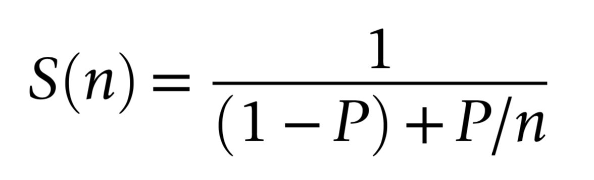
Amdahls "Law" : Expected Speedup Limited by Serial Processing

S(n) Expected Speedup

P

parallelizable proportion

1-P

non-parallelizable portion

n

parallel speedup factor

optical photon simulation, P ~ 99% of CPU time

• -> potential overall speedup S(n) is 100x
• even with parallel speedup factor >> 1500x

Must consider processing "big picture"

• remove bottlenecks one by one
• re-evaluate "big picture" after each

Amdahls "Law" : Expected Speedup Limited by Serial Processing Talk

The serial portion of processing determines the overall speedup because the parallel portion goes to zero

With neutrino telescopes I expect the situation will be more like 99.9% limited so there is potential for some really drastic overall speedups for you.

Understanding GPU Graphical Origins -> Effective GPU Computation

OpenGL Rasterization Pipeline

GPUs evolved to rasterize 3D graphics at 30/60 fps

• 30/60 "launches" per second, each handling millions of items
• literally billions of small "shader" programs run per second

Simple Array Data Structures (N-million,4)

• millions of vertices, millions of triangles
• vertex: (x y z w)
• colors: (r g b a)

Constant "Uniform" 4x4 matrices : scaling+rotation+translation

• 4-component homogeneous coordinates -> easy projection

Graphical Experience Informs Fast Computation on GPUs

• array shapes similar to graphics ones are faster
  • "float4" 4*float(32bit) = 128 bit memory reads are favored
  • Opticks photons use "float4x4" just like 4x4 matrices
• GPU Launch frequency < ~30/60 per second
  • avoid copy+launch overheads becoming significant
  • ideally : handle millions of items in each launch

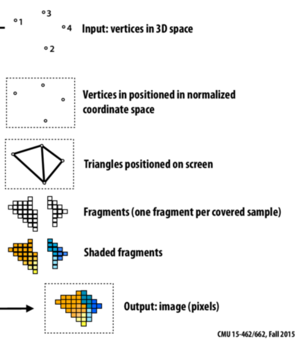
Understanding GPU Graphical Origins -> Effective GPU Computation Talk

Rasterization is the process of going from input 3D vertices which are collections of 4 floats to 2d pixel values.

GPUs evolved to do this rasterization.

When using GPUs you should keep these origins in mind.

• for example, copying or operating on float4s 4*32bits is faster that float3 128bits are better for alignment reasons
• graphics pipeline is based around 4x4 matrices and 4 component homogeneous coordinates
• graphics updates at something like 30/60 frames per second : so do not expect to do thousands of launches per second, each launch has overhead
• performance is gained by doing more in each launch

CPU Optimizes Latency, GPU Optimizes Throughput

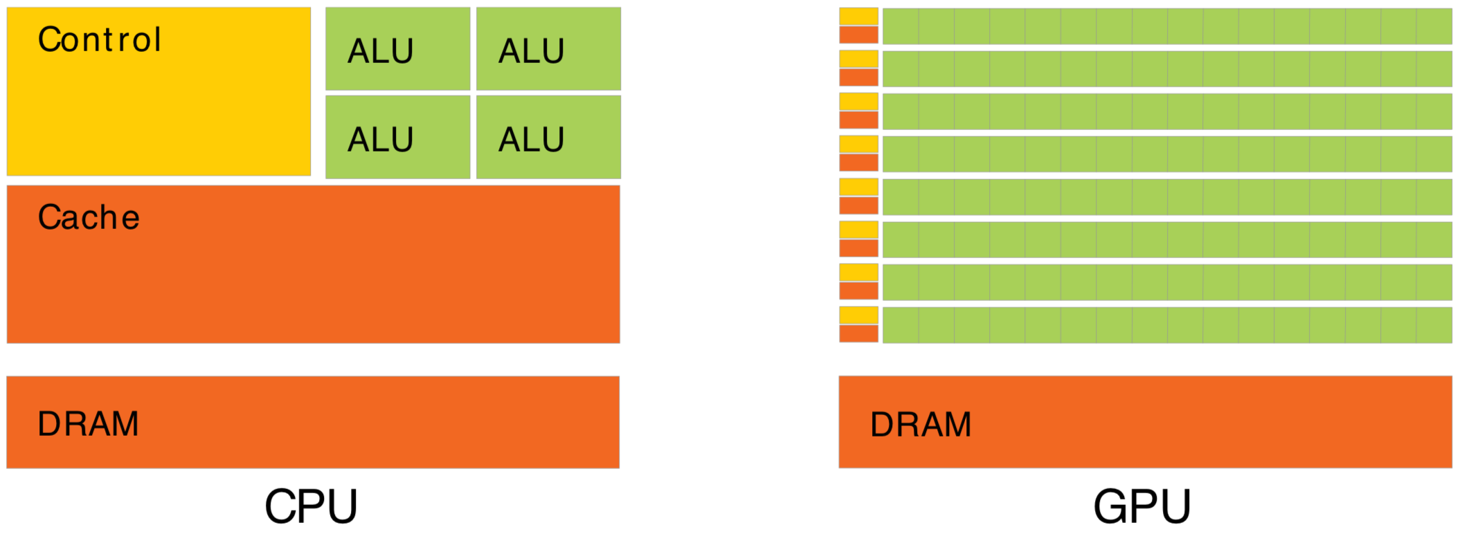
Waiting for memory read/write, is major source of latency...

CPU : latency-oriented : Minimize time to complete single task : avoid latency with caching

• complex : caching system, branch prediction, speculative execution, ...

GPU : throughput-oriented : Maximize total work per unit time : hide latency with parallelism

• many simple processing cores, hardware multithreading, SIMD (single instruction multiple data)
• simpler : lots of compute (ALU), at expense of cache+control
• can tolerate latency, by assuming abundant other tasks to resume : design assumes parallel workload

Totally different processor architecture -> Total reorganization of data and computation

• major speedups typically require total rethink of data structures and computation

CPU Optimizes Latency, GPU Optimizes Throughput Talk

Latency hiding works using hardware multi-threading, so when one group of threads is blocked waiting to read from global memory for example : other groups of threads are resumed.

This is only effective at hiding latency when there are enough other threads in flight at the same time.

If your processing is not parallel enough, you will not make effective use of the GPU

How to Make Effective Use of GPUs ? Parallel / Simple / Uncoupled

Abundant parallelism

• many thousands of tasks (ideally millions)

Low register usage : otherwise limits concurrent threads

• simple kernels, avoid branching

Little/No Synchronization

• avoid waiting, avoid complex code/debugging

Minimize CPU<->GPU copies

• reuse GPU buffers across multiple CUDA launches

How Many Threads to Launch ?

• can (and should) launch many millions of threads
  • largest Opticks launch : 400M threads, at VRAM limit
• maximum thread launch size : so large its irrelevant
• maximum threads inflight : #SM*2048 = 80*2048 ~ 160k
  • best latency hiding when launch > ~10x this ~ 1M

Understanding Throughput-oriented Architectures https://cacm.acm.org/magazines/2010/11/100622-understanding-throughput-oriented-architectures/fulltext

NVIDIA Titan V: 80 SM, 5120 CUDA cores

How to Make Effective Use of GPUs ? Parallel / Simple / Uncoupled Talk

The main things that dictate how effective your use of the GPU is going to be ...

• ideally you need to have many thousands of simple independent tasks to make best use of the GPU
• each task needs to be simple : low register usage and small stacksize : otherwise you limit the number of concurrent tasks
• idependence of the tasks really helps, as development is then much easier

Many people guess that you should launch only as many threads as there are cores in the GPU ... but thats wrong, you need to launch large multiples of that to get best performance

The reason is latency hiding, which only works when there is abundant parallelism, when the GPU workload resembles that from 3D graphics you will get best performance.

GPU Demands Simplicity (Arrays) -> Big Benefits : NumPy + CuPy

Separate address space -> cudaMemcpy -> Serialization

upload/download : host(CPU)<->device(GPU)

• Serialize everything -> Arrays
• Many small tasks -> Arrays
• Random Access/Order undefined -> Arrays

Object-oriented : mixes data and compute

• complicated serialization
• good for complex systems, up to ~1000 objects

Array-oriented : separate data from compute

• inherent serialization + simplicity
• good for millions of element systems

NumPy : standard array handling package

• simple .npy serialization
• read/write NumPy arrays from C++ https://github.com/simoncblyth/np/blob/master/NP.hh

https://realpython.com/numpy-array-programming/

GPU Demands Simplicity (Arrays) -> Big Benefits : NumPy + CuPy Talk

Simplicity requirement comes from the need to do many things in parallel and also from the need to serialize everything in order to copy it to GPU global memory.

This constraint means must use Arrays

But that comes with advantages:

• easy serialization
• use of standard tools like NumPy

Survey of High Level General Purpose CUDA Packages

CuPy : Simplest CUDA Interface

• https://cupy.chainer.org/
• NumPy API accelerated by CUDA stack
• plus some of SciPy API

• develop processing with NumPy on CPU
  • switch numpy->cupy to test on GPU
  • great for prototyping

"Production" CuPy ? Depends on requirements:

• integrations (eg Geant4, OpenGL, ...)
• control + performance

• Learn CUDA basics (kernels, thread+memory hierarchy, ...)
  • BUT: base development on higher level libs -> faster start

C++ Based Interfaces to CUDA

• Thrust : https://developer.nvidia.com/Thrust
  • C++ interface to CUDA performance
  • high-level abstraction : reduce, scan, sort
• CUB : http://nvlabs.github.io/cub/
  • CUDA C++ specific, GPU less hidden
• MGPU : https://github.com/moderngpu/moderngpu
  • teaching tool : examples of CUDA algorithms

Mature NVIDIA Basis Libraries

• cuRAND, cuFFT, cuBLAS, cuSOLVER, cuTENSOR, ...
  • https://developer.nvidia.com/gpu-accelerated-libraries

RAPIDS : New NVIDIA "Suite" of open source data science libs

• GPU-accelerated open source data science suite
  • "... end-to-end data science workflows..." http://rapids.ai/
  • cuDF : GPU dataframe library, Pandas-on-GPU

Survey of High Level General Purpose CUDA Packages Talk

This slide is here just to highlight some projects that provide a quick start at using CUDA.

CuPy implememnts the NumPy API ontop of the CUDA stack. It is a great way to get started with CUDA

CuPy is quite a new project you might not have heard of, it builds ontop of the NVIDIA CUDA stack and implements the NumPy API powered by a CUDA implementation.

Rendering Five Decades of Research 1

Rendering Five Decades of Research 1 Talk

Graphics rendering has come a long way over the past 50 years, starting from the first use of ray casting in 1968.

This illustrates some of the milestones on graphics rendering.

Rendering Five Decades of Research 2

Rendering Five Decades of Research 2 Talk

• Early rendering : mostly hacks : like rasterization
• techniques have become more and more physically based.
  • simpler, more consistent
  • better hardware has allows simpler approach
• the last milestone is NVIDIA RTX in 2018

Project Sol

Project Sol Talk

• this is a frame from an NVIDIA Demo video called "Project Sol"
• search for "Project Sol" to see the video
• movie frames can take hours to render
• so the surprise with Project Sol is that it runs in real time on a single GPU
• this is made possible by NVIDIA RTX:
  • dedicated GPU hardware for raytracing, texturing and AI-inference

Path Tracing in Production 1

Path Tracing in Production 1 Talk

Path tracing is short for : Monte Carlo Path Tracing

This is the abstract from a course held at the SIGGRAPH graphics conference

• Monte Carlo Path Tracing is now the standard rendering technique for movie production

Path Tracing in Production 2

Path Tracing in Production 2 Talk

For many movies:

• every frame is the result of monte carlo optical photon simulations, involving billions of photons

The Rendering Equation 1

The Rendering Equation 1 Talk

SMALL Computer graphics is all about finding solutions to the rendering equation.

The equation stems from energy conservation in equilibrium:

• Outgoing light in some direction comes from emission and reflection at the point
• Light reflected from the point depends on all the incoming light and the reflection characteristics of the surface.

The lines on the images try to illustrate that:

• what the eye at point x sees at some x-prime depends on inputs from all the x-double-prime and each double-prime point depends on all the treble-prime ones

You can see blue, green and red casts on the teapot coming from color bleeding : that arises from the multiple bounces or indirect lighting.

The rendering equation is a recursive integral equation

• surface properties are known
• what is unknown is the radiance distribution function

If you can solve it you can construct images from any viewpoint.

The Rendering Equation 2

The Rendering Equation 2 Talk

This form of recursive integral equation has a solution which is a sum of terms with progressively increasing bounces.

0. emission : looking at the light
1. direct illumination
2. one-bounce indirect illumination
3. two-bounce indirect illumination

Top row shows individual contributions, with the cumulative sum on the bottom row.

Recursive integral eqn -> sum of integrals

The "Volumetric Rendering Equation" is a generalization to cover participating media eg clouds, fire, fog, skin

Samples per Pixel 1

Samples per Pixel 1 Talk

Monte Carlo Path Tracing

• amazingly general technique
• can produce images indistinguisable from reality
• BUT : suffers from slow convergence

Samples per Pixel 2

Samples per Pixel 2 Talk

The technique has the usual monte carlo disadvantage of slow convergence. Much of computer graphics is about devising ways to bias the sampling and speed up the convergence.

NVIDIA OptiX AI Denoiser 1

NVIDIA OptiX AI Denoiser 1 Talk

NVIDIA OptiX includes a new AI based approach to removing noise.

NVIDIA OptiX AI Denoiser 2

https://research.nvidia.com/publication/interactive-reconstruction-monte-carlo-image-sequences-using-recurrent-denoising

NVIDIA OptiX AI Denoiser 2 Talk

This benefits from hardware dedicated to AI inferencing, the Tensor Cores.

Physically Based Rendering Book : www.pbr-book.org

Physically Based Rendering Book : www.pbr-book.org Talk

I hope I have got some of your interested to learn more about graphics. A good and very extensive book on physically based rendering is available for free at this url.

This book won an Oscar : for its usefulness to the film industry

Optical Simulation : Computer Graphics vs Physics

• handling of time is the crucial difference

Despite differences many techniques+hardware+software directly applicable to physics eg:

• GPU accelerated ray tracing (NVIDIA OptiX)
• GPU accelerated property interpolation via textures (NVIDIA CUDA)
• GPU acceleration structures (NVIDIA BVH)

Potentially Useful CG techniques for "billion photon simulations"

• irradiance caching, photon mapping, progressive photon mapping

[1] search for: "Volumetric Rendering Equation"

Optical Simulation : Computer Graphics vs Physics Talk

There are great similarities between graphics rendering and physics simulation but also some clear differences.

• principal difference is handling of time : graphics always assuming long time scales and equilibium
• despite the differences there is great scope for re-purposing computer graphics techniques+projects to assist physics simulation

Neutrino Telescope Optical Simulations : Giga-Photon Propagations

• Cherenkov light generation
• radioactive + biological backgrounds
• propagation : scattering + absorption (billions)
  • direct light (unscattered) : fast
  • indirect (scattered) : slow
• detection on sparse sensors

Opticks as drop in fast replacement for Geant4

Full+fast GPU accelerated simulation:

• Cerenkov generation, Rayleigh scattering, absorption
• angle dependent sensor collection efficiency culling
• BUT: launch size, VRAM limited: 48G ≈ 400M photons

Re-usage is caching optimization, still need full propagation:

• populate the cache
• validate the trickery
• re-usage reduces need for expensive propagations

Neutrino Telescope Optical Simulations : Giga-Photon Propagations Talk

SMALL 1st: full propagation

• Opticks as a drop in replacement for Geant4, needs work:
  • auto-split to fit in VRAM, multi-GPU
  • simpler geometry -> more speedup than JUNO

2nd: full propagation with "snapshots" for re-use (sidebar)

• split handling of direct and indirect light as very different.
• orient snapshot to different primaries -> avoid re-doing propagation
• just resume propagation near the sensors

DISADVANTAGE:

• need to devise snapshot/re-use approach + validate it
• "snapshots" will be large + not either-or need both + complex workflow
• When/where to snapshot (sidebar)

Opticks Rayleigh Scattering : CUDA line-by-line port of G4OpRayleigh

130 __device__ void rayleigh_scatter(Photon &p, curandState &rng)
131 {
137     float3 newDirection, newPolarization ;
139     float cosTheta ;
141     do {
145         newDirection = uniform_sphere(&rng);
146         rotateUz(newDirection, p.direction );
151
152         float constant = -dot(newDirection,p.polarization);
153         newPolarization = p.polarization + constant*newDirection ;
154
155         // newPolarization
156         // 1. transverse to newDirection (as that component is subtracted)
157         // 2. same plane as old p.polarization and newDirection (by construction)
158         // 
...         ... corner case elided ...
182         if(curand_uniform(&rng) < 0.5f) newPolarization = -newPolarization ;
184
185         newPolarization = normalize(newPolarization);
189         cosTheta = dot(newPolarization,p.polarization) ;
190
191     } while ( cosTheta*cosTheta < curand_uniform(&rng)) ;
192
193     p.direction = newDirection ;
194     p.polarization = newPolarization ;
195 }

Have to persist the polarization vector, to truly resume a propagation

• could persist pre-scatter : polarization, direction

https://bitbucket.org/simoncblyth/opticks/src/master/optixrap/cu/rayleigh.h

Opticks Rayleigh Scattering : CUDA line-by-line port of G4OpRayleigh Talk

SMALL Have to persist the polarization vector, to truly resume a propagation. As the angle between polarization vectors before and after scatters follows a cos-squared distribution.

Not doing so will prevent strict validation.

Collecting photons at scatters duplicates less. The post-scatter direction and polarization is generated from the pre-scatter values : better to store pre.

Developing a photon "snapshot" cache

Where/when/what to collect ?

• tetrahedral volumetric meshes (tet-mesh)
  • inherent segmentation
  • natural adaptive resolution
  • triangle faces : Giga-rays/s intersection (RT Cores)[1]
  • good for general light field capture
• "concentric" spheres/cylinders/cones oriented to primary
  • natural for exploiting track axis rotational symmetry
• at scatters (pre-scatter/post-scatter parameters)
  • position, direction, polarization
  • can generate post from pre, but not v.v.
• collect photons OR aggregate binned PDFs ?
  • PDF->CDF->generate photons (like Opticks "gensteps")

Too many options: experimentation needed to iterate towards solution

[1] RTX Beyond Ray Tracing: Exploring the Use of Hardware Ray Tracing Cores for Tet-Mesh Point Location https://www.willusher.io/publications/rtx-points

Developing a photon "snapshot" cache Talk

Too many open questions: experimentation needed to iterate towards solution

• requires fast spatial lookup such as kd-tree.
• For efficient use with Opticks will need a CUDA implementation that can work within the OptiX model.
• the ones in blue, are what I would try first
• I favor those because they are similar to the graphics technique of photon mapping : and I expect I could find a CUDA implementation to make a quickstart at them
• tetrahedral mesh would be interesting for the general case of snapshoting the photon field, but simulating photons from primaries has symmetries
• voxel grid good for simplicity, large, sparse

Photon Mapping 1

Photon Mapping 1 Talk

The graphics technique of photon mapping is an old from from around 2001. It collects photons into a kd-tree which is a space partitioning data structure designed to speed up spatial queries.

Balancing the tree has the advantage that you can then easily serialize it and traverse it just by bit manipulations on the array index.

This is just one example of spatial data structures, searches might reveal some CUDA implementation that would lead me to trying another approach.

Photon Mapping 2

Photon Mapping 2 Talk

To learn more about photon mapping, this is the classic book on the subject. The lower link is a 200 page course on photon mapping.

• I pick this example as its well documented, with many open source implementations.
• There are enhancements and similar things that might be better.
• But it will be easier to understand those after you are familiar with the original photon mapping and kd-trees.

Conclusion

Opticks : state-of-the-art GPU ray tracing applied to optical photon simulation and integrated with Geant4, eliminating memory and time bottlenecks.

• neutrino telescope simulation can benefit drastically from Opticks
  • Drastic speedup -> better detector understanding -> greater precision
  • more photon limited -> more overall speedup ( 99.9% -> 1000x )
  • graphics : rich source of techniques, inspiration, CUDA code to try

Conclusion Talk

So in summary : Opticks applies the best available GPU ray tracing to optical photon simulation resulting in speedups exceeding three orders of magnitude.

Neutrino telescope simulation is so extremely limited by the photons that there is potential for large overall speedups.

The field of graphics has lots of potential to provide techniques and code for working with really large photon propagations.